travel time graph for p and s waves

Powerful math software that is easy to use

• Maple Add-Ons

Advanced System Level Modeling

• MapleSim Add-Ons

Systems Engineering

• Consulting Services

Maple T.A. and Möbius

Automotive and Aerospace

Machine design & industrial automation.

• Application Areas
• Product Pricing
• Institutional Student Licensing
• Maplesoft Elite Maintenance (EMP)
• Product Training
• Online Product Help
• Webinars & Events
• Publications
• Content Hubs
• Examples & Applications
• About Maplesoft
• Media Center
• User Community

• Maple Learn
• Maple Calculator App
• System Engeneering
• Online Education Products

Online Help

All products    maple    maplesim.

The second type of wave to consider when determining the epicenter of an earthquake is the S-wave . These waves are also referred to as secondary or shear waves. S-waves can also be characterized by some unique properties:

The following animation helps to understand the motion of each type of wave.

A seismogram  is the graph output from a seismograph , which is used to determine the epicenter of an earthquake. When consulting the seismogram, P-waves always appear before S-waves, as they travel faster and can travel through three states of matter as opposed to one.

To determine the distance of an earthquake epicenter:

Suppose the P-wave arrives at t  = 1.0 min and the S-wave arrives at t  = 6.0 min. Determine the distance of the earthquake epicenter given the following information.

Download Help Document

Download a Free Trial of Maple

Try Maple free for 15 days with no obligation.

Maple 2024 now available.

Save an additional 20% on Maple 2024 Upgrades until March 31, 2024.

Want to create or adapt books like this? Learn more about how Pressbooks supports open publishing practices.

12.2 Seismic Waves and Measuring Earthquakes

The shaking from an earthquake travels away from the rupture in the form of seismic waves . Seismic waves are measured to determine the location of the earthquake, and to estimate the amount of energy released by the earthquake (its magnitude ).

Types of Seismic Waves

Seismic waves are classified according to where they travel, and how they move particles.

Seismic waves that travel through Earth’s interior are called body waves . P-waves are body waves that move by alternately compressing and stretching materials in the direction the wave moves. For this reason, P-waves are also called compression waves. The “P” in P-wave stands for primary, because P-waves are the fastest of the seismic waves. They are the first to be detected when an earthquake happens.

A P-wave can be simulated by fixing one end of a spring to a solid surface, then giving the other end a sharp push toward the surface (Figure 12.8, top).  The compression will propagate (travel) along the length of the spring. Some parts of the spring will be stretched, and others compressed. Any one point on the spring will jiggle forward and backward as the compression travels along the spring.

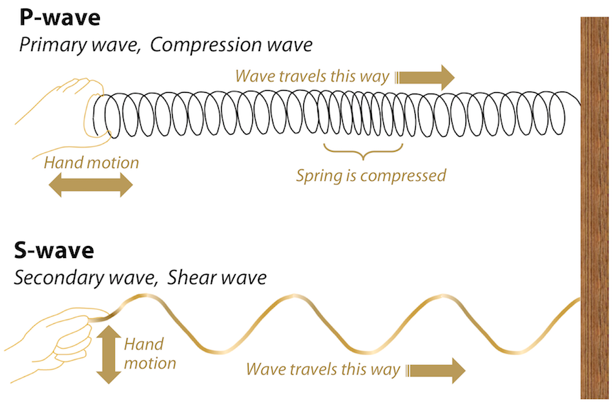
S-waves are body waves that move with a shearing motion, shaking particles from side to side. S-waves can be simulated by fixing one end of a rope to a solid surface, then giving the other end a flick (Figure 12.8, bottom). Any one point on the rope will move from side to side at a right angle to the direction in which the snaking motion is traveling. The “S” in S-wave stands for secondary, because S-waves are slower than P-waves, and are detected after the P-waves are measured. S-waves cannot travel through liquids.

P-waves and S-waves can travel rapidly through geological materials, at speeds many times the speed of sound in air.

Surface Waves

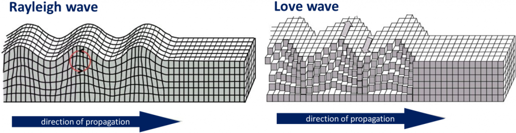
When body waves reach Earth’s surface, some of their energy is transformed into surface waves, which travel along Earth’s surface. Two types of surface waves are Rayleigh waves and Love waves (Figure 12.9). Rayleigh waves (R-waves) are characterized by vertical motion of the ground surface, like waves rolling on water. Love waves (L-waves) are characterized by side-to-side motion. Notice that the effects of both kinds of surface waves diminish with depth in Figure 12.9.

Surface waves are slower than body waves, and are detected after the body waves. Surface waves typically cause more ground motion than body waves, and therefore do more damage than body waves.

Concept Check: Seismic Wave Types

Fill in the blanks to complete this summary of types of seismic waves.

              -waves ( hint: P, S, R, or L?) are               ( hint: fast or slow?) body waves that move by compressing and stretching rock.

              -waves ( hint: P, S, R, or L?) are               ( hint: fast or slow?) body waves that move by shearing rock.

              -waves ( hint: P, S, R, or L?) are surface waves that produce a rolling motion.

              -waves ( hint: P, S, R, or L?) are surface waves that produce a side-to-side motion.

To check your answers, navigate to the below link to view the interactive version of this activity.

Recording Seismic Waves Using a Seismograph

A seismometer is an instrument that detects seismic waves. An instrument that combines a seismometer with a device for recording the waves is called a seismograph . The graphical output from a seismograph is called a seismogram . Figure 12.10 (right) shows how a seismograph works. The instrument consists of a frame or housing that is firmly anchored to the ground. A mass is suspended from the housing, and can move freely on a spring. When the ground shakes, the housing shakes with it, but the mass remains fixed. A pen attached to the mass moves up and down on a rotating drum of paper, drawing a wavy line, the seismogram. The seismograph in Figure 12.10 (right) is oriented to measure vertical ground motion. The photo on the left shows a seismograph oriented to record horizontal ground motion.

The pen and drum of a mechanical seismograph record the motion of the ground relative to the mass. However, unless an earthquake causes a large amount of ground motion directly beneath the seismograph, the height of the wave recorded on paper might be very small, making the seismogram difficult to analyze. The seismograph on the right has a device to amplify the ground motion, drawing larger waves that are easier to study.

Modern seismographs record shaking as electrical signals, and are able to transmit those signals. This means seismologists need not return to the instrument to collect recordings before the records can be examined.

Finding The Location of an Earthquake

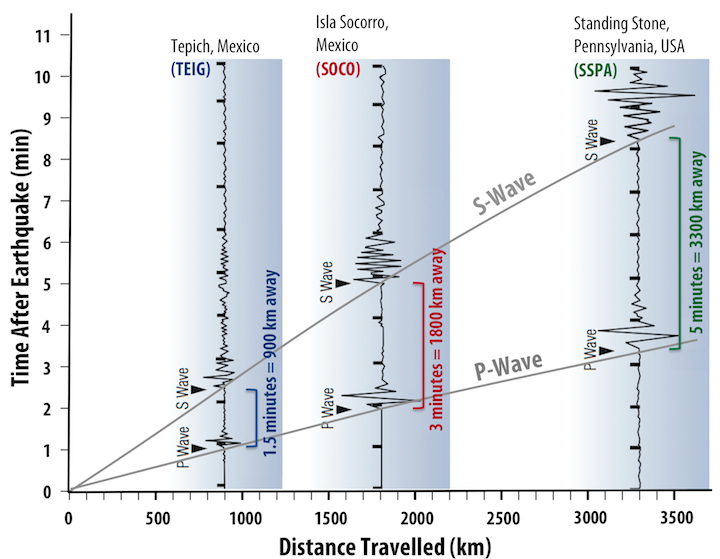
P-waves travel faster than S-waves. As the waves travel away from the location of an earthquake, the P-wave gets farther and farther ahead of the S-wave. Therefore, the farther a seismograph is from the location of an earthquake, the longer the delay between when the P-wave arrival is recorded, and the S-wave arrival is recorded. The delay between the P-wave and S-wave arrival appears as a widening gap in a diagram of P-wave and S-wave travel times (Figure 12.11, grey lines).

P-wave and S-wave arrival times can be identified on seismograms. In the three seismograms in Figure 12.11, the arrivals of the P-waves and S-waves are marked with arrows, and the interval in minutes between the P-wave and S-wave arrivals are noted. The seismograms were recorded at three different seismic stations (earthquake monitoring locations equipped with seismographs). The distance of each station from the earthquake is determined by finding the distance along the graph where the gap between the P-wave and S-wave travel-time curves matches the delay between P-wave and S-wave arrivals on the seismogram.

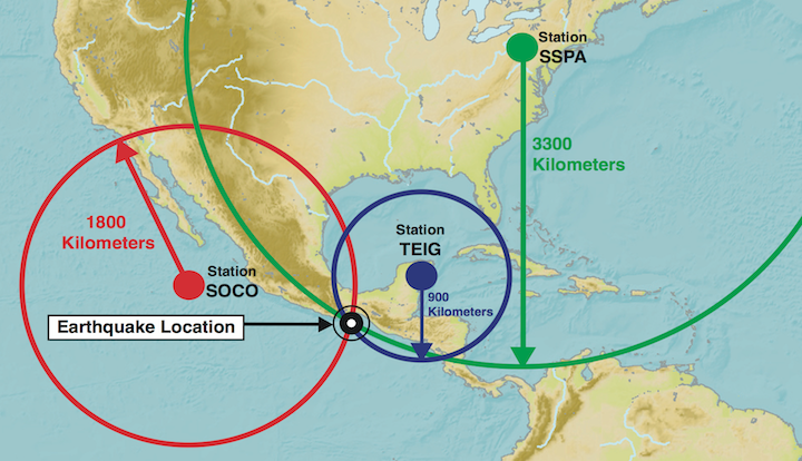
The delay between the P-wave and S-wave arrival at a seismic station can indicate how far the station is from the source of the earthquake, but not the direction the seismic waves came from. The possible locations of the earthquake can be represented on a map by drawing a circle around the seismic station, with the radius of the circle being the distance determined from the P-wave and S-wave travel times (Figure 12.12). If this is done for at least three seismic stations, the circles will intersect at the origin of the earthquake. This method is called triangulation .

Concept Check: Finding the Location of an Earthquake

Fill in the blanks to complete this description of how earthquakes are located by triangulation.

The               -waves ( hint: P or S) generated by an earthquake are faster than               -waves ( hint: P or S). The farther seismic waves have to travel before reaching a seismic                ( hint: a monitoring location with a seisometer), the more the fast waves will gain on the slow ones, and the longer we have to wait after the fast waves arrive to see the slow ones. We can use that lag to figure out how far away the earthquake was.

This information gives us the               ( hint: direction or distance?) to the earthquake, but not the               ( hint: direction or distance?). To find the actual location, we need the lag information measured from at least               ( hint: how many?) locations. Then we can draw a circle from each location with a radius that matches the               ( hint: direction or distance?) we figured out. The location of the earthquake is where all of the circles                ( hint: geometry term for crossing).

How Big Was It?

Earthquakes can be described in terms of their magnitude , which reflects the amount of energy released by the shaking. They can also be described in terms of intensity , which characterizes the impact of the shaking on people and their surroundings.

Earthquake Magnitude

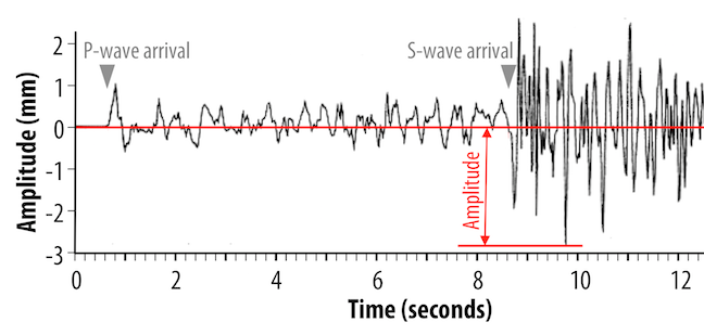
Earthquake magnitudes are determined by measuring the amplitudes of seismic waves. The amplitude is the height of the wave relative to the baseline (Figure 12.13). Wave amplitude depends on the amount of energy carried by the wave. The amplitudes of seismic waves reflect the amount of energy released by earthquakes.

The Richter magnitude scale uses the amplitudes of S-waves, and corrects for the decrease in amplitude that happens as the waves travel away from their source. The correction depends on how seismic waves interact with the specific rock types through which they travel, and therefore on local conditions, so the Richter magnitude is also referred to as the local magnitude .

While news reports about earthquakes might still refer to the “Richter scale” when describing magnitudes, the number they report is most likely the moment magnitude . The moment magnitude is calculated from the seismic moment of an earthquake. The seismic moment takes into account the surface area of the region that ruptured, how much displacement occurred, and the stiffness of the rocks. Moment magnitude can capture the difference between short earthquakes and longer ones resulting from larger ruptures, even of both types of earthquakes generate the same amplitude of waves. The moment magnitude scale is also better for earthquakes that are far from the seismic station. Seismic wave measurements are still used to determine the moment magnitude, however different waves are used than for the local magnitude scale.

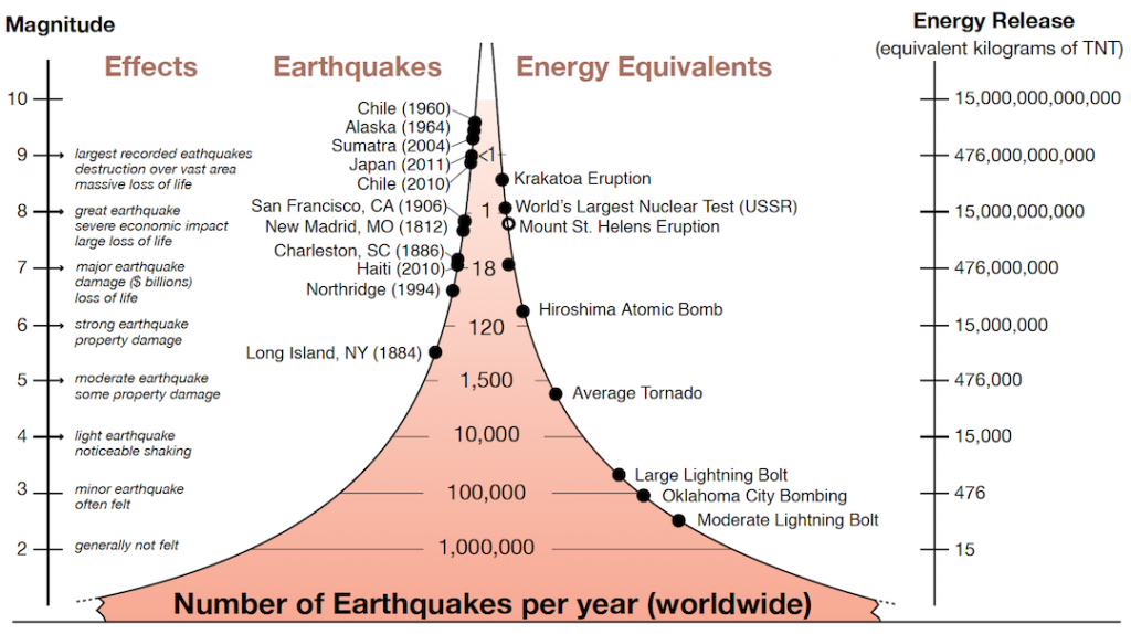
The magnitude scale is a logarithmic one rather than a linear one- an increase of one unit of magnitude corresponds to a 32 times increase in energy release (Figure 12.14). There are far more low-magnitude earthquakes than high-magnitude earthquakes. In 2017 there were 7 earthquakes of M7 (magnitude 7) or greater, but millions of tiny earthquakes.

Earthquake Intensity

Intensity scales were first used in the late 19th century, and then adapted in the early 20th century by Giuseppe Mercalli and modified later by others to form what we now call the Modified Mercalli Intensity Scale (Table 12.1). To determine the intensity of an earthquake, reports are collected about what people felt and how much damage was done. The reports are then used to assign intensity ratings to regions where the earthquake was felt.

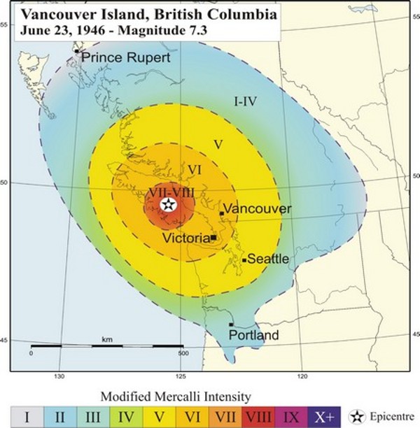
Intensity values are assigned to locations, rather than to the earthquake itself. This means that intensity can vary for a given earthquake, depending on the proximity to the epicentre and local conditions. For the 1946 M7.3 Vancouver Island earthquake, intensity was greatest in the central island region (Figure 12.15). In some communities within this region, chimneys were damaged on more than 75% of buildings. Some roads were made impassable, and a major rock slide occurred. The earthquake was felt as far north as Prince Rupert, as far south as Portland Oregon, and as far east as the Rockies, but with less intensity.

Intensity estimates are important as a way to identify regions that are especially prone to strong shaking. A key factor is the nature of the underlying geological materials. The weaker the underlying materials, the more likely it is that there will be strong shaking. Areas underlain by strong solid bedrock tend to experience far less shaking than those underlain by unconsolidated river or lake sediments.

An example of this effect is the 1985 M8 earthquake that struck the Michoacán region of western Mexico, southwest of Mexico City. There was relatively little damage near the epicentre, but 350 km away in heavily populated Mexico City there was tremendous damage and approximately 5,000 deaths. The reason is that Mexico City was built largely on the unconsolidated and water-saturated sediment of former Lake Texcoco. These sediments resonate at a frequency of about two seconds, which was similar to the frequency of the body waves that reached the city. Consequently, the shaking was amplified.  Survivors of the disaster recounted that the ground in some areas moved up and down by approximately 20 cm every two seconds for over two minutes. Damage was greatest to buildings between 5 and 15 storeys tall, because they also resonated at around two seconds, which amplified the shaking.

Try It: Modified Mercalli Intensity Scale

Ammon, C. J. (2001). Earthquake size . http://eqseis.geosc.psu.edu/~cammon/HTML/Classes/IntroQuakes/Notes/earthquake_size.html

• Source: U. S. Geological Survey (1989). The severity of an earthquake . USGS General Interest Publication, 1989-288-913 ↵

Physical Geology - H5P Edition Copyright © 2021 by Karla Panchuk is licensed under a Creative Commons Attribution-NonCommercial-ShareAlike 4.0 International License , except where otherwise noted.

Share This Book

9.2 Measuring Earthquakes

The shaking from an earthquake travels away from the rupture in the form of seismic waves . Seismic waves are measured to determine the location of the earthquake, and to estimate the amount of energy released by the earthquake (its magnitude ).

Types of Seismic Waves

Seismic waves are classified according to where they travel, and how they move particles.

Seismic waves that travel through Earth’s interior are called body waves . P-waves are body waves that move by alternately compressing and stretching materials in the direction the wave moves. For this reason, P-waves are also called compression waves. The “P” in P-wave stands for primary, because P-waves are the fastest of the seismic waves. They are the first to be detected when an earthquake happens.

A P-wave can be simulated by fixing one end of a spring to a solid surface, then giving the other end a sharp push toward the surface (Figure 9.8, top).  The compression will propagate (travel) along the length of the spring. Some parts of the spring will be stretched, and others compressed. Any one point on the spring will jiggle forward and backward as the compression travels along the spring.

S-waves are body waves that move with a shearing motion, shaking particles from side to side. S-waves can be simulated by fixing one end of a rope to a solid surface, then giving the other end a flick (Figure 9.8, bottom). Any one point on the rope will move from side to side at a right angle to the direction in which the snaking motion is traveling. The “S” in S-wave stands for secondary, because S-waves are slower than P-waves, and are detected after the P-waves are measured. S-waves cannot travel through liquids.

P-waves and S-waves can travel rapidly through geological materials, at speeds many times the speed of sound in air.

Surface Waves

When body waves reach Earth’s surface, some of their energy is transformed into surface waves, which travel along Earth’s surface. Two types of surface waves are Rayleigh waves and Love waves (Figure 9.9). Rayleigh waves (R-waves) are characterized by vertical motion of the ground surface, like waves rolling on water. Love waves (L-waves) are characterized by side-to-side motion. Notice that the effects of both kinds of surface waves diminish with depth in Figure 9.9.

Surface waves are slower than body waves, and are detected after the body waves. Surface waves typically cause more ground motion than body waves, and therefore do more damage than body waves.

Recording Seismic Waves Using a Seismograph

A seismometer is an instrument that detects seismic waves. An instrument that combines a seismometer with a device for recording the waves is called a s eismograph . The graphical output from a seismograph is called a seismogram . Figure 9.10 (right) shows how a seismograph works. The instrument consists of a frame or housing that is firmly anchored to the ground. A mass is suspended from the housing, and can move freely on a spring. When the ground shakes, the housing shakes with it, but the mass remains fixed. A pen attached to the mass moves up and down on a rotating drum of paper, drawing a wavy line, the seismogram. The seismograph in Figure 9.10 (right) is oriented to measure vertical ground motion. The photo on the left shows a seismograph oriented to record horizontal ground motion.

The pen and drum of a mechanical seismograph record the motion of the ground relative to the mass. However, unless an earthquake causes a large amount of ground motion directly beneath the seismograph, the height of the wave recorded on paper might be very small, making the seismogram difficult to analyze. The seismograph on the right has a device to amplify the ground motion, drawing larger waves that are easier to study.

Modern seismographs record shaking as electrical signals, and are able to transmit those signals. This means seismologists need not return to the instrument to collect recordings before the records can be examined.

Finding The Location of an Earthquake

P-waves travel faster than S-waves. As the waves travel away from the location of an earthquake, the P-wave gets farther and father ahead of the S-wave. Therefore, the farther a seismograph is from the location of an earthquake, the longer the delay between when the P-wave arrival is recorded, and the S-wave arrival is recorded. The delay between the P-wave and S-wave arrival appears as a widening gap in a diagram of P-wave and S-wave travel times (Figure 9.11, grey lines).

P-wave and S-wave arrival times can be identified on seismograms. In the three seismograms in Figure 9.11, the arrivals of the P-waves and S-waves are marked with arrows, and the interval in minutes between the P-wave and S-wave arrivals are noted. The seismograms were recorded at three different seismic stations (earthquake monitoring locations equipped with seismographs). The distance of each station from the earthquake is determined by finding the distance along the graph where the gap between the P-wave and S-wave travel-time curves matches the delay between P-wave and S-wave arrivals on the seismogram.

The delay between the P-wave and S-wave arrival at a seismic station can indicate how far the station is from the source of the earthquake, but not the direction from which the seismic waves travelled. The possible locations of the earthquake can be represented on a map by drawing a circle around the seismic station, with the radius of the circle being the distance determined from the P-wave and S-wave travel times (Figure 9.12). If this is done for at least three seismic stations, the circles will intersect at the origin of the earthquake.

How Big Was It?

Earthquakes can be described in terms of their magnitude , which reflects the amount of energy released by the shaking. They can also be described in terms of intensity , which characterizes the impact of the shaking on people and their surroundings.

Earthquake Magnitude

Earthquake magnitudes are determined by measuring the amplitudes of seismic waves. The amplitude is the height of the wave relative to the baseline (Figure 9.13). Wave amplitude depends on the amount of energy carried by the wave. The amplitudes of seismic waves reflect the amount of energy released by earthquakes.

The Richter magnitude scale uses the amplitudes of S-waves, and corrects for the decrease in amplitude that happens as the waves travel away from their source. The correction depends on how seismic waves interact with the specific rock types through which they travel, and therefore on local conditions, so the Richter magnitude is also referred to as the local magnitude .

While news reports about earthquakes might still refer to the “Richter scale” when describing magnitudes, the number they report is most likely the moment magnitude . The moment magnitude is calculated from the seismic moment of an earthquake. The seismic moment takes into account the surface area of the region that ruptured, how much displacement occurred, and the stiffness of the rocks. Moment magnitude can capture the difference between short earthquakes and longer ones resulting from larger ruptures, even of both types of earthquakes generate the same amplitude of waves. The moment magnitude scale is also better for earthquakes that are far from the seismic station. Seismic wave measurements are still used to determine the moment magnitude, however different waves are used than for the local magnitude scale.

The magnitude scale is a logarithmic one rather than a linear one- an increase of one unit of magnitude corresponds to a 32 times increase in energy release (Figure 9.14). There are far more low-magnitude earthquakes than high-magnitude earthquakes. In 2017 there were 7 earthquakes of M7 (magnitude 7) or greater, but millions of tiny earthquakes.

Earthquake Intensity

Intensity scales were first used in the late 19th century, and then adapted in the early 20th century by Giuseppe Mercalli and modified later by others to form what we now call the Modified Mercalli Intensity Scale (Table 9.1). To determine the intensity of an earthquake, reports are collected about what people felt and how much damage was done. The reports are then used to assign intensity ratings to regions where the earthquake was felt.

Intensity values are assigned to locations, rather than to the earthquake itself. This means that intensity can vary for a given earthquake, depending on the proximity to the epicenter and local conditions. For the 1946 M7.3 Vancouver Island earthquake, intensity was greatest in the central island region (Figure 9.15). In some communities within this region, chimneys were damaged on more than 75% of buildings. Some roads were made impassable, and a major rock slide occurred. The earthquake was felt as far north as Prince Rupert, as far south as Portland Oregon, and as far east as the Rockies, but with less intensity.

Intensity estimates are important as a way to identify regions that are especially prone to strong shaking. A key factor is the nature of the underlying geological materials. The weaker the underlying materials, the more likely it is that there will be strong shaking. Areas underlain by strong solid bedrock tend to experience far less shaking than those underlain by unconsolidated river or lake sediments.

An example of this effect is the 1985 M8 earthquake that struck the Michoacán region of western Mexico, southwest of Mexico City. There was relatively little damage near the epicenter, but 350 km away in heavily populated Mexico City there was tremendous damage and approximately 5,000 deaths. The reason is that Mexico City was built largely on the unconsolidated and water-saturated sediment of former Lake Texcoco. These sediments resonate at a frequency of about two seconds, which was similar to the frequency of the body waves that reached the city. Consequently, the shaking was amplified.  Survivors of the disaster recounted that the ground in some areas moved up and down by approximately 20 cm every two seconds for over two minutes. Damage was greatest to buildings between 5 and 15 stories tall, because they also resonated at around two seconds, which amplified the shaking.

Video: Geoscience Videos – Measuring Earthquakes

Ammon, C. J. (2001). Earthquake Size Visit website

Licenses and Attributions

“Physical Geology, First University of Saskatchewan Edition” by Karla Panchuk is licensed under CC BY-NC-SA 4.0 Adaptation: Renumbering

https://openpress.usask.ca/physicalgeology/

Principles of Earth Science Copyright © 2021 by Katharine Solada and K. Sean Daniels is licensed under a Creative Commons Attribution-NonCommercial-ShareAlike 4.0 International License , except where otherwise noted.

Share This Book

• Earthquake Center
• Regional Information
• Learning & Education
• Research & Monitoring
• Additional Resources

Home » Earthquake Center

• Latest Earthquakes
• - EQ Notification Service
• - Feeds & Data
• - Animations
• Recent Earthquakes
• Historic Earthquakes
• - "Top 10" Lists & Maps
• - Significant EQs
• - Earthquake Search
• - EQ Summary Posters
• - Scientific Data
• About EQ Maps
• Did You Feel It?
• Energy & Broadband Solutions
• Fast Moment Tensors
• Seismogram Displays

Earthquake Travel Time Information and Calculator

• Specify Earthquake
• Graph of seismic travel time in minutes versus distance in degrees for an earthquake at the Earth's surface
• Table of P and S minus P times versus distance in degrees
• Composite ANSS list of earthquakes for the past 14 days
• Site Search

• school Campus Bookshelves
• menu_book Bookshelves
• perm_media Learning Objects
• login Login
• how_to_reg Request Instructor Account
• hub Instructor Commons
• Download Page (PDF)
• Download Full Book (PDF)
• Periodic Table
• Physics Constants
• Scientific Calculator
• Reference & Cite
• Tools expand_more
• Readability

selected template will load here

This action is not available.

13.4: Locating an Earthquake Epicenter

• Last updated
• Save as PDF
• Page ID 5696

• Deline, Harris & Tefend
• University of West Georgia via GALILEO Open Learning Materials

During an earthquake, seismic waves are sent all over the globe. Though they may weaken with distance, seismographs are sensitive enough to still detect these waves. In order to determine the location of an earthquake epicenter, seismographs from at least three different places are needed for a particular event. In Figure 13.9, there is an example seismogram from a station that includes a minor earthquake. 

Once three seismographs have been located, find the time interval between the arrival of the P-wave and the arrival of the S-wave. First, determine the P-wave arrival, and read down to the bottom of the seismogram to note at what time (usually marked in seconds) that the P-wave arrived. Then do the same for the S-wave. The arrival of seismic waves will be recognized by an increase in amplitude – look for a pattern change as lines get taller and more closely spaced (ex. Figure 13.10).

By looking at the time between the arrivals of the P- and S-waves, one can determine the distance to the earthquake from that station, with longer time intervals indicating longer distance. These distances are determined using a travel-time curve, which is a graph of Pand S-wave arrival times (see Figure 13.11).

Though the distance to the epicenter can be determined using a travel-time graph, the direction cannot be told. A circle with a radius of the distance to the quake can be drawn. The earthquake occurred somewhere along that circle. Triangulation is required to determine exactly where it happened. Three seismographs are needed. A circle is drawn from each of the three different seismograph locations, where the radius of each circle is equal to the distance from that station to the epicenter. The spot where those three circles intersect is the epicenter (Figure 13.12).

To successfully complete the Unit Activity, you will need to know how to use seismic data to locate the epicenter of an earthquake. The following activity will help you to understand how seismologists calculate the location of an earthquake and will also help you with the Unit Activity.

You will need to use graphing paper in order to complete Part II of this Learning Activity.

Learning Activity

Part i: using a travel-time graph to determine distance to the epicenter.

Use the travel-time graph to answer the following questions.

• Complete the following table:
• Determine the arrival times for P and S waves for earthquake epicenters located at a distance of:
• 3,000 km P wave: 5 min. 40 s., S wave: 10 min 10 s.
• 9,500 km P wave: 12 min. 30 s., S wave: 22 min. 50 s.
• What would the time delay between P and S waves be for an earthquake whose epicenter distance was:
• 8,000 km approximately 9 minutes and 20 seconds
• 2,000 km approximately 3 minutes and 5 seconds

Part II: Locating the epicenter of an earthquake using triangulation

Data from one seismograph station will allow us to draw a circle whose radius equals the distance from the station to the earthquake. The epicenter for the earthquake could be anywhere on this circle. Data from a second seismograph station allows us to draw a second circle. This second circle intersects the first circle at two points, narrowing our epicenter down to two possible locations. Data from a third seismograph station is necessary to accurately determine the epicenter. The epicenter will be located where the three circles intersect. This process of using three separate data sets in geology to locate one unique common point is called triangulation .

You will need to use graphing paper in order to complete this exercise.

• Label a sheet of graphing paper so that the coordinates along both the x- and y-axes go from at least –10 to 10.
• Seismic Station A is located at grid coordinate (0,3). Plot this point on your grid and clearly label it. Station A receives a signal (i.e. the time difference between the arrival of the P and S waves) that indicates that an earthquake occurred at a distance of 6 units away from the receiving station. Now carefully draw a circle with a radius of 6 units around Station A.
• Station B is located at (–5,–5). Plot the location of Station B. Station B’s signal indicates that the earthquake occurred 5 units away. Draw in a circle with a radius of 5 units around Station B.
• What are the two possible grid locations (x- and y-coordinates) for the earthquake? The earthquake is located at one of two points where the circles around stations A and B intersect, either (–5.2,0) or (–0.5,–2.9).
• Station C is located at (3.2,–5) and its signal indicates that the earthquake is 4.2 units away. Again, plot the station location and a circle around the station showing the possible location of the earthquake.
• Examine your graph carefully, and determine the exact grid location for the location of the earthquake’s epicenter. All three circles intersect uniquely at (–0.5,–2.9). This is the location of the earthquake’s epicenter.

EarthScope Triangulation Map iris.edu/app/triangulation

• The Earthquake Triangulation app provides a simple interactive map where students or instructors can estimate the location of an earthquake using the distances between the earthquake and 3 or more seismic stations. The application allows users to place their choice of seismic stations on the maps and then enter the distances to the earthquake. Distance circles then appear on the map and the user can determine the likely earthquake location. Earthquake-station distances need to be calculated separately by first picking P and S arrival times on seismograms, and then using a P and S wave travel time graph to determine the distance.
• We are showing the 1000 latest earthquakes with a magnitude of at least 5.
• To plot a different selection of events, visit Interactive Earthquake Browser (IEB) . Using IEB’s filters, create the desired view, copy that URL and paste it here under Advanced Options > Paste IEB link here' and press enter or click on the map.
• To add a station’s S minus P time distance circle, click on the + Station button in the top right corner.
• You can adjust the position and the diameter the station by entering values manually, or by dragging the center of the created circle.
• Please send me an email if you have any questions or suggestions.

Station List: