travel graphs igcse

Ultimate Guide to Travel Graphs| Cambridge IGCSE Mathematics

Kulni gamage.

• Created on July 20, 2023

[Please watch the video attached at the end of this blog for a visual explanation on the Ultimate Guide to Travel Graphs]

Travel graphs fall under the bigger topic of Algebra, but unlike the other lessons under this topic, this is really simple and easy to understand… as long as you read the question carefully and pay attention to the readings of the graphs ?!

What is a travel graph?

A travel graph is a line graph that tells us how much distance has been covered by the object in question within a particular time. We can use travel graphs to represent the motion of cars, people, trains, buses, etc. This means travel graphs can tell us whether an object is still (stationary), moving at a constant speed, accelerating, or decelerating.  The y -axis represents the distance travelled while the x -axis shows the time it takes to travel a distance such as that.

James went on a cycling ride. The travel graph shows James’s distance from home on this cycle ride. Find James’s speed for the first 60 minutes.

We are told that James is going on a cycling ride and that the distance he travelled is what is shown here. What is required of us is to find James’s speed for the first 60 minutes. This means you need to mark the point at 60 minutes on the x -axis as shown in the picture below.

We have learnt when learning about Speed, Time and Distance that speed = distance/ time.

Therefore, in a distance-time graph, the slope that we see (also called the gradient) is what will give us the speed.

We can see that this particular cycle has travelled 12 km in 60 minutes.

When we substitute these values into the formula above, it would look like this:

When this formula is solved, then we get James’s speed for the first 60 minutes , which is 0.2 km/min .

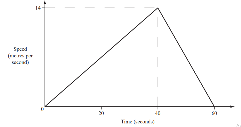
A train journey takes one hour. The diagram shows the speed-time graph for this journey. Calculate the total distance of this journey.

We need to be careful here because this time what we have in this question is a speed-time graph and not a distance-time graph.

In a speed-time graph, the gradient of a slope represents either acceleration or deceleration, which will be concepts touched upon in later lessons. The distance travelled is found by calculating the area under a speed-time graph.

In order to calculate the distance travelled by the train therefore, we need to calculate the area under the graph that is drawn. To make things easier, we can separate this graph into shapes:

2 triangles and 1 rectangle

Triangle 1: Area of a triangle = ½ × base of triangle × height of triangle Area = ½ × 4 km × 3 km/min Area = 6 km2

Rectangle: Length of the rectangle can be found by finding out the difference between 50 and 4, which equals to 46 min. The height of the rectangle is 3 km/min. Area = length × base Area = 46 min × 3 km/min Area = 138 km

Triangle 2: Area of a triangle = ½ × base of triangle × height of triangle Area = ½ × 10 km × 3 km/min Area = 15 km

Total Area under the graph = Total distance travelled by the train Therefore, Total Distance = Triangle 1 + Rectangle + Triangle 2 Total Distance = 6 km + 138 km + 15 km Total Distance =  159 km

Those are the basic tips and tricks you would need to learn in this particular chapter!

Travel Graphs at Exams

Pay attention to what sort of graph is given to you. Is it a distance-time graph? A speed-time graph? Depending on the type of graph, remember, the value represented by the gradient changes, and so does the value represented by the area under the graph.

Practice as many questions as you can on this topic. They are quite simple once you get the hang of them. You can find some questions in this quiz to check where you stand!

If you are struggling with IGCSE revision or the Mathematics subject in particular, you can reach out to us at Tutopiya to join revision sessions or find yourself the right tutor for you.

Watch the video below for a visual explanation of the lesson on the ultimate guide to travel graphs!

See author's posts

Recent Posts

• Top 10 Reasons to Choose Edexcel IGCSE: Global Recognition, Flexible Curriculum & More
• Tutopiya Unveils AI Tutor for IGCSE Maths Exams
• Educate and Empower: Subscribe to Tutopiya, Gift Education to Africa
• IGCSE Curriculum: Top 10 Benefits for Students
• Edexcel IGCSE: Benefits, Subjects, Syllabus, Pricing, and Tips for Edexcel IGCSE Success
• Navigating the AI Education Landscape: Trends in Singapore
• IGCSE Tutors Dubai: Affordable Group Classes, Boost Grades, Expert Tutors, Proven Results
• Empowering Minds: The Inspiring Journey of Fathima Safra Azmi
• Mastering IGCSE: Ace Your Exams in 3 Months with Our Unlimited Learning Program
• IGCSE Exam 2024 Revision: 10 Tips and Tricks to Score A*

Get Started

Learner guide

Tutor guide

Curriculums

IGCSE Tuition

PSLE Tuition

SIngapore O Level Tuition

Singapore A Level Tuition

SAT Tuition

Math Tuition

Additional Math Tuition

English Tuition

English Literature Tuition

Science Tuition

Physics Tuition

Chemistry Tuition

Biology Tuition

Economics Tuition

Business Studies Tuition

French Tuition

Spanish Tuition

Chinese Tuition

Computer Science Tuition

Geography Tuition

History Tuition

TOK Tuition

Privacy policy

22 Changi Business Park Central 2, #02-08, Singapore, 486032

All rights reserved

©2022 tutopiya

Travel Graphs

This section covers travel graphs, speed, distance, time, trapezium rule and velocity.

Speed, Distance and Time

The following is a basic but important formula which applies when speed is constant (in other words the speed doesn't change):

Remember, when using any formula, the units must all be consistent. For example speed could be measured in m/s, distance in metres and time in seconds.

If speed does change, the average (mean) speed can be calculated: Average speed = total distance travelled                              total time taken

In calculations, units must be consistent, so if the units in the question are not all the same (e.g. m/s, m and s or km/h, km and h), change the units before starting, as above.

The following is an example of how to change the units:

Change 15km/h into m/s. 15km/h = 15/60 km/min               (1) = 15/3600 km/s = 1/240 km/s      (2) = 1000/240 m/s = 4.167 m/s        (3)

In line (1), we divide by 60 because there are 60 minutes in an hour. Often people have problems working out whether they need to divide or multiply by a certain number to change the units. If you think about it, in 1 minute, the object is going to travel less distance than in an hour. So we divide by 60, not multiply to get a smaller number.

If a car travels at a speed of 10m/s for 3 minutes, how far will it travel? Firstly, change the 3 minutes into 180 seconds, so that the units are consistent. Now rearrange the first equation to get distance = speed × time. Therefore distance travelled = 10 × 180 = 1800m = 1.8km

Velocity and Acceleration

Velocity is the speed of a particle and its direction of motion (therefore velocity is a vector quantity, whereas speed is a scalar quantity).

When the velocity (speed) of a moving object is increasing we say that the object is accelerating . If the velocity decreases it is said to be decelerating. Acceleration is therefore the rate of change of velocity (change in velocity / time) and is measured in m/s².

A car starts from rest and within 10 seconds is travelling at 10m/s. What is its acceleration?

Distance-Time Graphs

These have the distance from a certain point on the vertical axis and the time on the horizontal axis. The velocity can be calculated by finding the gradient of the graph. If the graph is curved, this can be done by drawing a chord and finding its gradient (this will give average velocity) or by finding the gradient of a tangent to the graph (this will give the velocity at the instant where the tangent is drawn).

Velocity-Time Graphs/ Speed-Time Graphs

A velocity-time graph has the velocity or speed of an object on the vertical axis and time on the horizontal axis. The distance travelled can be calculated by finding the area under a velocity-time graph. If the graph is curved, there are a number of ways of estimating the area (see trapezium rule below). Acceleration is the gradient of a velocity-time graph and on curves can be calculated using chords or tangents, as above.

The distance travelled is the area under the graph. The acceleration and deceleration can be found by finding the gradient of the lines.

On travel graphs, time always goes on the horizontal axis (because it is the independent variable).

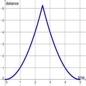
Trapezium Rule

This is a useful method of estimating the area under a graph. You often need to find the area under a velocity-time graph since this is the distance travelled.

Area under a curved graph = ½ × d × (first + last + 2(sum of rest))

d is the distance between the values from where you will take your readings. In the above example, d = 1. Every 1 unit on the horizontal axis, we draw a line to the graph and across to the y axis. 'first' refers to the first value on the vertical axis, which is about 4 here. 'last' refers to the last value, which is about 5 (green line).] 'sum of rest' refers to the sum of the values on the vertical axis  where the yellow lines meet it. Therefore area is roughly: ½ × 1 × (4 + 5 + 2(8 + 8.8 + 10.1 + 10.8 + 11.9 + 12 + 12.7 + 12.9 + 13 + 13.2 + 13.4)) = ½ × (9 + 2(126.8)) = ½ × 262.6 = 131.3 units²

iGCSE Mathematics (0580) :E2.10 Interpret and use graphs in practical situations including travel graphs and conversion graphs.iGCSE Style Questions Paper 2

iGCSE Physics iGCSE Maths iGCSE Chemistry iGCSE Biology

The diagram shows the speed-time graph of a bus journey between two bus stops. Hamid runs at a constant speed of 4m/s along the bus route. He passes the bus as it leaves the first bus stop. The bus arrives at the second bus stop after 60 seconds. How many metres from the bus is Hamid at this time?

Ans: 180 www 

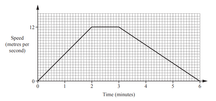
A tram leaves a station and accelerates for 2 minutes until it reaches a speed of 12 metres per second. It continues at this speed for 1 minute. It then decelerates for 3 minutes until it stops at the next station. The diagram shows the speed-time graph for this journey. Calculate the distance, in metres, between the two stations.

Ans: 2520 m

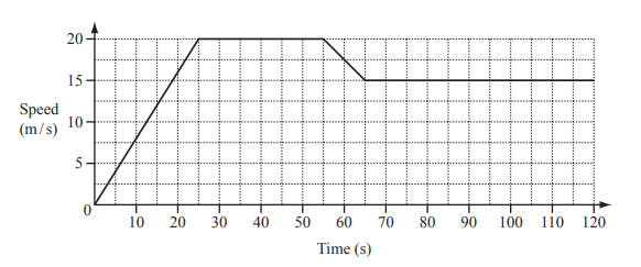
The diagram shows the speed-time graph for the first 120 seconds of a car journey. (a) Calculate the acceleration of the car during the first 25 seconds.

(b) Calculate the distance travelled by the car in the first 120 seconds.

(a) 2.8 oe \(m/s^2\) (b) 700 m

A car travels at 56km/h. Find the time it takes to travel 300 metres. Give your answer in seconds correct to the nearest second.

Ans: 19 nfww

A train travels for m minutes at a speed of x metres per second. (a) Find the distance travelled, in kilometres, in terms of m and x. Give your answer in its simplest form. ………………………………….. km

(b) When m = 5, the train travels 10.5km. Find the value of x. x = …………………………………………

(a) \(\frac{3mx}{50}\) or 0.06 mx (b) 35

0.8 or \(\frac{4}{5}\)

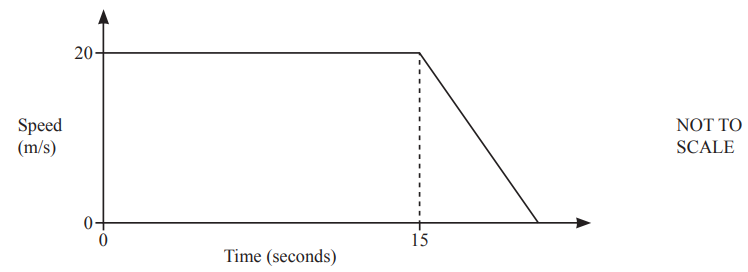
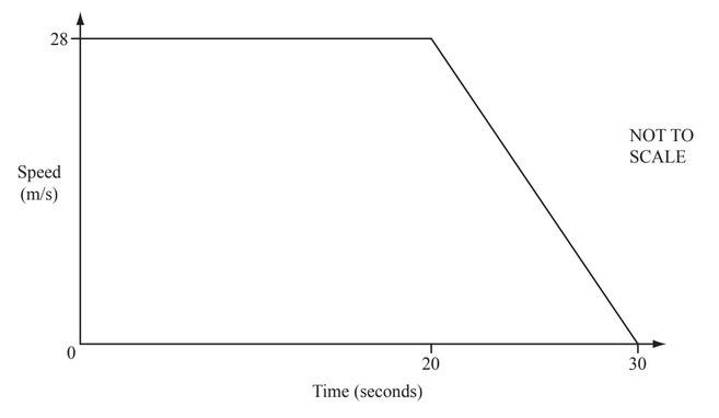
A car travels at 20m/s for 15 seconds before it comes to rest by decelerating at 2.5m/s 2 .

Find the total distance travelled.

(a) Find the acceleration of the train. ……………………………………m/\(s^2\)

(b) Calculate the distance the train has travelled in this time. Give your answer in kilometres. …………………………………….. km

(a) 0.25 or \(\frac{1}{4}\) (b) 0.45

Diagonal line from (0, 0) to (30, 12) and Horizontal line from (30, 12) to (70, 12)

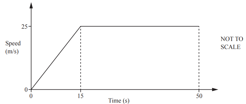
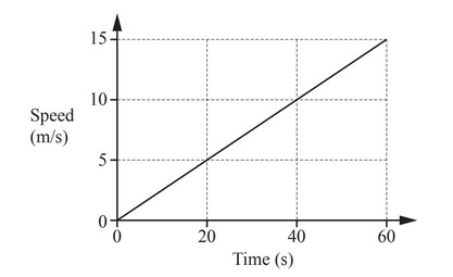
The speed–time graph shows the first 50 seconds of a journey.

(a) the acceleration during the first 15 seconds,

__ m/s 2 [1]

(b) the distance travelled in the 50 seconds.

22(a) \(1\frac{2}{3}\) or 1.67 or 1.666 to 1.667

22(b) 1062.5

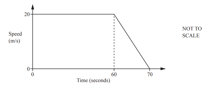
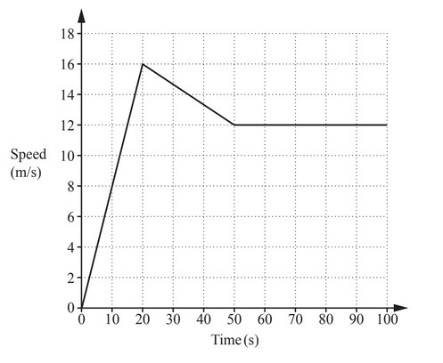
The diagram shows information about the final 70 seconds of a car journey.

(a) Find the deceleration of the car between 60 and 70 seconds.

(b) Find the distance travelled by the car during the 70 seconds.

The diagram shows the speed–time graph for 100 seconds of the journey of a car and of a motorbike. (a) Find the deceleration of the car between 60 and 100 seconds. ………………………………….. \(m/s^{2}\) (b) Calculate how much further the car travelled than the motorbike during the 100 seconds. ……………………………………… m

(a) 0.3 (b) 360

The diagram shows the speed–time graph for 90 seconds of a journey. Calculate the total distance travelled during the 90 seconds. ……………………………………… m

A hummingbird beats its wings 24 times per second.

(a) Calculate the number of times the hummingbird beats its wings in one hour.

(b) Write your answer to part(a) in standard form

(a) Using unitary method ,

1 sec = 24 times

60\(\times\) 60 sec = 24\(\times\)3600

 = 86400 times

(b)  Standard form basically means writing the numbers in the power of 10 

So, 86400 in standard form is : 8.64\(\times 10^4\)

A train leaves Barcelona at 21:28 and takes 10 hours and 33 minutes to reach Paris. (a) Calculate the time the next day when the train arrives in Paris.

(b) The distance from Barcelona to Paris is 827 km. Calculate the average speed of the train in kilometres per hour.

(a)  21:28 is 9:28 pm  in 12 hours format clock

So, Adding 10 hours 33 minutes to 9:28 pm gives 8:01 am 

So, the train will be reaching by 8:01 ,the next day

(b) Average speed=\(\frac{ Total distance}{Total time}/)

Now , 10 hours 33 minutes= 10+33/60 minutes=10.5 hours 

So, putting it into formula :

Average speed= \(\frac{ 827km}{10.5hours}/)

=78.38 km/hour

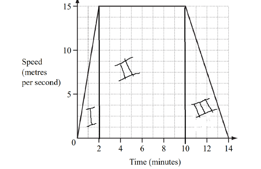
The diagram shows the speed-time graph of a train journey between two stations. The train accelerates for two minutes, travels at a constant maximum speed, then slows to a stop. (a) Write down the number of seconds that the train travels at its constant maximum speed.

(b) Calculate the distance between the two stations in metres.

(c) Find the acceleration of the train in the first two minutes. Give your answer in m/s2

=0(120)+\(\frac{1}{2}\times\frac{5}{8}\times 120\times 120

Distance is II= 15m/s\(\times (8\times 60\)

15\(\times 480\)

Similarly , Distance is III=180-450

Total distance =900+72300+1350m

(c) a=\(\frac{\Delta V}{\Delta V}\)

a=\(\frac{V_f-V_i}{T_f-T_i}\)

a=\(\frac{15-0}{(2.60)-0}\)

=\(\frac{1}{8}\) m/\(s^2)\)

A container ship travelled at 14 km/h for 8 hours and then slowed down to 9 km/h over a period of 30 minutes. It travelled at this speed for another 4 hours and then slowed to a stop over 30 minutes. The speed-time graph shows this voyage.

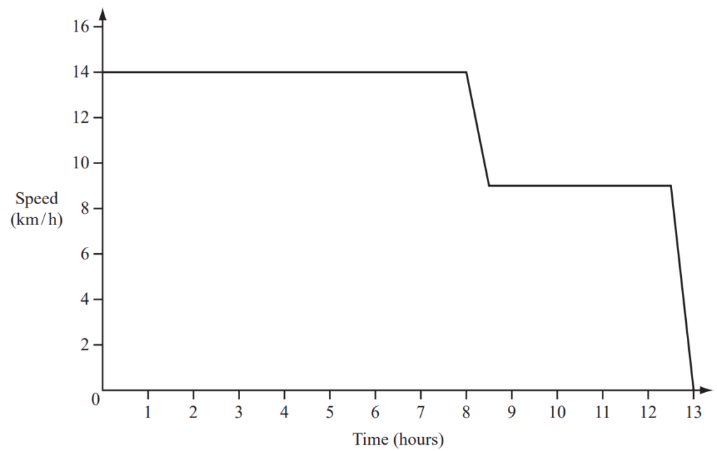
(a) Calculate the total distance travelled by the ship.

(b) Calculate the average speed of the ship for the whole voyage.

(a) Distance = speed \(\times time\)

A person in a car, travelling at 108 kilometres per hour, takes 1 second to go past a building on the side of the road. Calculate the length of the building in metres.

To calculate the length of the building. We can use the formula, Distance \(= Speed \times Time\) Given that the speed of the car is 108 kilometers per hour and the time taken to go past the building is 1 second, we need to convert the speed from kilometers per hour to meters per second. 1 kilometer = 1000 meters 1 hour = 3600 seconds Converting the speed, 108 kilometers per hour\(=\frac{108\times 1000 m}{3600 s}=30ms^{-1}\) Now, we can calculate the distance covered by the car in 1 second: \(Distance = Speed\times Time = 30 ms^{-1}\times 1s =\) 30 meters Therefore, the length of the building is 30 meters.

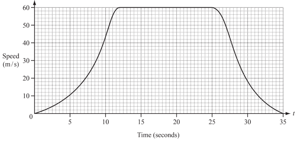
The graph shows the speed of a sports car after $t$ seconds. It starts from rest and accelerates to its maximum speed in 12 seconds.(a) (i) Draw a tangent to the graph at $t=7$. (ii) Find the acceleration of the car at $t=7$.

(b) The car travels at its maximum speed for 13 seconds. Find the distance travelled by the car at its maximum speed.

(a) (i) Tangent (ii) 4.4 to 6 (b) 780

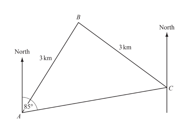
A, B and C are three places in a desert. Tom leaves A at 06 40 and takes 30 minutes to walk directly to B, a distance of 3 kilometres. He then takes an hour to walk directly from B to C, also a distance of 3 kilometres.

(a) At what time did Tom arrive at C?

(b) Calculate his average speed for the whole journey.

(c) The bearing of C from A is 085°. Find the bearing of A from C.

(a) (0)810 or 8:10 etc.

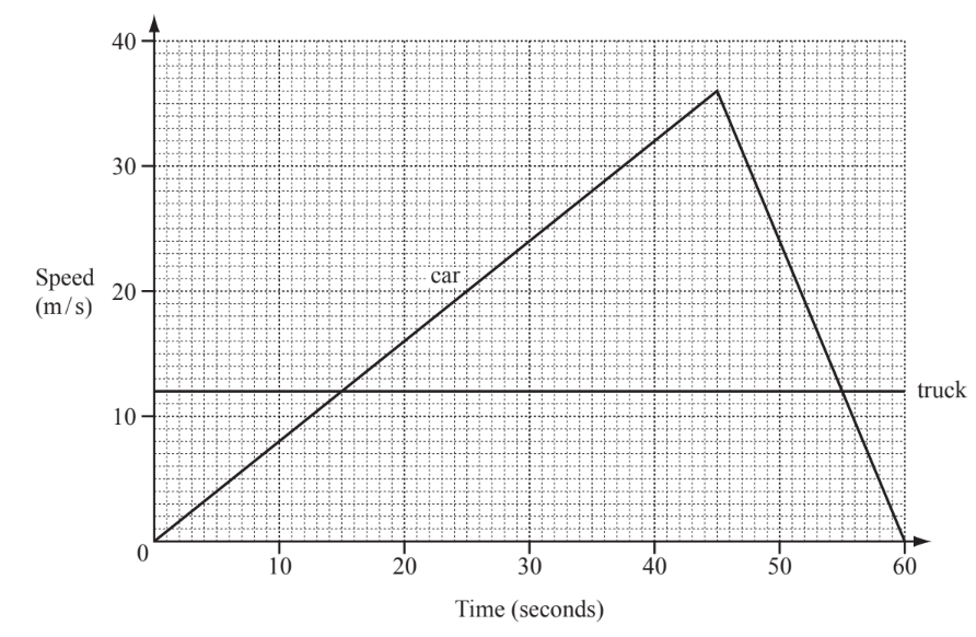
The graph shows the speed of a truck and a car over 60 seconds. (a) Calculate the acceleration of the car over the first 45 seconds.

(b) Calculate the distance travelled by the car while it was travelling faster than the truck.

(a) 0.8 or 4/5 cao

(b) 960 www

TOM ROCKS MATHS

Maths, but not as you know it…, gcse maths: travel graphs (speed-distance-time).

Learn how to use travel graphs relating speed, distance and time to solve problems. Tom introduces the topic, Bobby applies it to Usain Bolt’s 100-metre world record, and Susan uses an interactive tool on GeoGebra – go to www.geogebra.org/m/ABuBYdX7 to join in at home. 

This is the second lesson in a new series with the Maths Appeal duo – Bobby Seagull and Susan Okereke – and Tom Rocks Maths where we’ll be exploring the GCSE Maths syllabus to show the world that maths is accessible to everyone!

Watch Bobby and Susan answer YOUR questions here .

Watch Tom’s livestream here .

Share this:

• Click to share on Twitter (Opens in new window)
• Click to share on Facebook (Opens in new window)
• Click to share on Reddit (Opens in new window)
• Click to share on LinkedIn (Opens in new window)
• Click to email a link to a friend (Opens in new window)
• Click to share on Pinterest (Opens in new window)
• Click to share on WhatsApp (Opens in new window)
• Click to share on Tumblr (Opens in new window)

[…] Watch the video for lesson 2 (Travel graphs) here. […]

[…] Watch the video lesson here. […]

Leave a comment Cancel reply

• Already have a WordPress.com account? Log in now.
• Subscribe Subscribed
• Copy shortlink
• Report this content
• View post in Reader
• Manage subscriptions
• Collapse this bar

• International
• Schools directory
• Resources Jobs Schools directory News Search

STP Mathematics : Travel graphs ( (KS3, Year 9, IGCSE)

Subject: Mathematics

Age range: 11-14

Resource type: Worksheet/Activity

Last updated

4 November 2020

• Share through email
• Share through twitter
• Share through linkedin
• Share through facebook
• Share through pinterest

Learning Objectives • Finding distance from a graph • The relationship of speed, distance and time • Journeys with several parts • Drawing travel graphs • Getting information from travel graphs

Creative Commons "Sharealike"

Your rating is required to reflect your happiness.

It's good to leave some feedback.

Something went wrong, please try again later.

kathybailey

Thank you for sharing

Empty reply does not make any sense for the end user

I could use some of the questions

the worksheets were useful but how would you correct the answers without an answer key.....

Report this resource to let us know if it violates our terms and conditions. Our customer service team will review your report and will be in touch.

Not quite what you were looking for? Search by keyword to find the right resource:

Cambridge IGCSE Mathematics

Website by Oliver Bowles, Richard Wade & Jim Noble

Updated 6 March 2024

InThinking Subject Sites

Subscription websites for Cambridge IGCSE teachers & their classes

Find out more

• thinkigcse.net
• IGCSE Economics
• IGCSE Geography
• IGCSE History

InThinking Subject Sites for Cambridge IGCSE Teachers and their Classes

Supporting igcse educators.

• Comprehensive help & advice on teaching IGCSE.
• Written by experts with vast subject knowledge.
• Innovative ideas on ATL & pedagogy.
• Detailed guidance on all aspects of assessment.

Developing great materials

• More than one million words across 4 sites.
• Masses of ready-to-go resources for the classroom.
• Dynamic links to current affairs & real world issues.
• Updates every week 52 weeks a year.

Integrating student access

• Give your students direct access to relevant site pages.
• Single student login for all of your school’s subscriptions.
• Create reading, writing, discussion, and quiz tasks.
• Monitor student progress & collate in online gradebook.

Meeting schools' needs

• Global reach with thousands of users worldwide.
• Use our materials to create compelling unit plans.
• Save time & effort which you can reinvest elsewhere.
• Consistently good feedback from subscribers.

For information about pricing, click here

Download brochure

• Travel Graphs
• Algebra and Graphs
• All Activities

How can you describe your position? What happens when you move?

Can you describe this movement?

This is a really fun practical activity that will get you to do just that.

Students using a motion sensor to track their 'journey' and reproduce travel graphs.

Part A - Practical

In the activity below, the idea is to try and reproduce the journeys that were made by the person who recorded these journeys in the first place. The graphs describe the position of a person as time passes. The journeys are made over a few seconds and a few metres.

With Motion Sensors

Part B - Speed vs Time

In this second activity students are asked to make the link between distance-time graphs and speed-time graphs.

• Print out and cut up the graphs from this sheet.
• Match a graph with a number (distance-time) with a graph with a letter (speed-time).
• Some of these graphs have been left blank for you to complete!
• As an extension, students could find formula for some of the graphs.

Measurement of Permeability

Fundamentals of fluid flow in porous media, permeability:.

The permeability of a porous medium can be determined from the samples extracted from the formation or by in place testing such as well logging and well testing. Measurement of permeability in the case of isotropic media is usually performed on linear, mostly cylindrical shaped, “core” samples. Cores are cylinders with approximately 3.81cm (1.5 inch) diameter and 5 cm (2 inch) length. Sometimes the permeability tests run on a whole core samples about 30-50 cm long. The experiment can be arranged so as to have horizontal or vertical flow through the sample. Permeability is reduced by overburden pressure, and this factor should be considered in estimating permeability of the reservoir rock in deep wells because permeability is an anisotropic property of the porous rock, that is, it is directional. Routine core analysis is generally concerned with plug samples drilled parallel to bedding planes and, hence, parallel to the direction of flow in the reservoir. These yield horizontal permeabilities ( K h ). The measured permeabilities on plugs that are drilled perpendicular to the bedding planes are referred to as vertical permeability ( K v ). Both liquids and gases have been used to measure permeability. However liquids sometimes change the pore structure and therefore the permeability. For example injection of water to a sample with some amount of clay leads to decreasing permeability due to swelling of the clays.  There are several factors that could lead to some of error in determining reservoir permeability. Some of these factors are:

• Core sample may not be representative of the reservoir rock because of reservoir heterogeneity.
• Core recovery may be incomplete.
• Permeability of the core may be altered when it is cut, or when it is cleaned and dried in preparation for analysis. This problem is likely to occur when the rock contains reactive clays.

As core samples usually contain water and oil, it is necessary to prepare the core samples for the test. Cores are dried in an oven or extracted by a Soxhlet extractor and then they are subsequently dried. The residual fluids are thus removed and the core samples become 100% saturated with air. In principle measurement at a steady single flow rate permits the “routine” calculation of the permeability from Darsy’s law. The core is inserted in a core holder. A pressure applied on the surface of the core as confining pressure. An appropriate pressure gradient is adjusted across the core sample and the rate of flow of air through the plug is observed. The permeability could be found from either equation (2‑32) or (2‑33). However there is considerable experimental error in this experiment so the requirement that permeability be determined for conditions of viscous flow is best satisfied by obtaining data at several flow rates and plotting the flow rate versus pressure drop, as shown in Figure 2‑25.  A straight line is fitted to the data points. According to the Darcy’s law, the slope of this line is K / μ , and this line must pass through the origin. But at ultralow flow rates, the flow rate is not proportional to pressure drop. Darcy’s law should not be extrapolated to the origin. Deviation from the straight line at high flow rates is an indication of turbulent flow (Figure 2‑25). This deviation shows that the pressure drop in turbulent flow is higher than viscous flow. By increasing the pressure drop we can reach to a maximum flow rate capacity of the medium, after that flow rate will not increase by increasing the pressure drop.

The same experiment can be done with water or other liquids. In this case the core sample should be fully saturated with the testing liquid. When liquid is used as the testing fluid, care must be taken that it does not react with the solids in the core sample. The permeability of a core sample measured by flowing air is always greater than the permeability obtained when a liquid is the flowing fluid. Klinkenberg (1941) postulated, on the basis of his laboratory experiments, that liquids had a zero velocity at the sand grain surface, while gases exhibited some finite velocity at the sand grain surface. This resulted in a higher flow rate for the gas at a given pressure differential.

Correction can be applied for the change in permeability because the reduction in confining pressure on the sample.

Example 2-6 The following data obtained during a routine permeability test at 70 o F. Find the permeability.

• Flow rate = 2000 cc of air at 1 atm in 400 sec
• Downstream pressure = 1 atm
• Viscosity of air at test temperature = 0.02 cP
• Core cross sectional area = 3 cm 2
• Core length = 5 cm
• Upstream Pressure = 1.75 atm

Measurements of permeability on large core samples generally yield better indication of permeability of limestone than do with small core sample. Rocks which contain fractures in situ separate along natural plane of weakness when cored. Therefore the conductivity of such fractures will not be included in the laboratory data.

Effect of reactive liquid on permeability

While water used as testing liquid in permeability determination, in samples with clay material water act as a reactive liquid in connection with permeability determination. Reactive liquids alter the internal geometry of the porous medium which causes permeability change. The effect of clay swelling in presence of water when water used as testing fluid in permeability test is the most known effect of a reactive testing fluid. The degree of swelling is a function of water salinity. While the fresh water may cause swelling of the cementation material in the core it is a reversible process. Highly saline water can pass through the core and return the permeability to its original value.

The Klinkenberg Effect

This variation caused by “gas slippage” phenomenon. The phenomenon of gas slippage occurs when the diameter of the capillary opening approaches the mean free path of the gas. As mentioned before in flowing of the gas through the porous media the velocity at the solid wall cannot, in general, be considered zero, but a so called “slip” or “drift” velocity at the wall must be taken into account. This effect becomes significant when the mean free path of the gas molecules is of comparable magnitude as the pore size. When the mean free path is such smaller than the pore size, the slip velocity becomes negligibly small. As in liquids the mean free path of molecules is of the order of the molecular diameter, so the no-slip condition always applied in liquid flow.

The mean free path of a gas is a function of molecular size and the kinetic energy of the gas. Therefore the “Klinkenberg Effect” is a function of the gas that is used as testing fluid and the conditions of the test like as pressure and temperature. Figure 2‑26 is a plot of the permeability of the porous medium as determined at various mean pressures using hydrogen, nitrogen and carbon monoxide as the testing fluids.

Note that for each gas a straight line is observed for the observed permeability as a function of 1 / P m . The data obtained with lowest molecular weight gas yields the straight line with greater slop, indicative of a greater slippage effect. All the line when extrapolated to infinite mean pressure, ( 1 / P m = 0 ), intercept the permeability axes at a common point. This point is the equivalent liquid permeability, K L .

It is established that the permeability of a porous medium to a single phase liquid is equal to the equivalent liquid permeability.

The magnitude of the Klinkenberg effect varies with the core permeability as well as type of the gas used in the experiment as shown in Figure 2‑27.

• b = Klinkenberg factor
• K g = measured gas permeability
• P m = mean pressure
• K L = equivalent liquid permeability, i.e., absolute permeability, k
• m = slope of the line
• b = constant for a given gas in a given medium

Klinkenberg suggested that the “Klinkenberg factor” is a function of:

• Type of the gas used in measuring the permeability
• Pore throat size distribution

• K i = initial guess of the absolute permeability, md
• K i+1 = new permeability value to be used for the next iteration
• i = iteration level
• f ( K i ) = Equation 2-44 as evaluated by using the assumed value of K i .
• f ́ ( K i ) = first-derivative of Equation (2‑44) as evaluated at K i

Example (2-7) The permeability of a core plug is measured by air. Only one measurement is made at a mean pressure of 2.152 psi. The air permeability is 46.6 md. Estimate the absolute permeability of the core sample. Compare the result with the actual absolute permeability of 23.66 md.

Assume ki = 30 and apply the Newton-Raphson method to find the required solution as shown below.

After three iterations, the Newton-Raphson method converges to an absolute value for the permeability of 22.848 md.

Effect of overburden pressure

All the confining forces release and rock matrix expands when the core is removed from the formation. Fluid flow path in the rock changes by expansion of the rock’s matrix. Compaction of the core due to the overburden pressure may cause as much as 60% reduction in the permeability of various formations. So there is a need to an empirical correlation to correct the surface permeability for overburden pressure. It is noted that some formations are more compressible than others, so we need more data to develop this correlation.

Forscheimer Equation

ADD TEXT TO SECTION (Section Not Complete)

<<  FRACTURE SYSTEM PERMEABILITY

SATURATION >>

Cities [ edit ]

• 58.013889 56.248889 1 Perm — the capital is a major industrial city with nearly one million residents
• 57.433333 56.933333 5 Kungur — a small 17th century city with some fine 18th century architecture; near the Belogorsky Monastery and excellent spelunking opportunities in the Kungur Ice Cave

Other destinations [ edit ]

Understand [ edit ].

Perm, the capital, is the main attraction in Perm Krai, which sees travelers coming through on the Trans-Siberian Railway .

Talk [ edit ]

See Russian phrasebook .

Get in [ edit ]

There are three international flights per week to Perm ( PEE  IATA ) from Frankfurt (6 hours). Domestic flights arrive daily from Moscow (2 hours) and nearby Yekaterinburg . Flights from Saint Petersburg are less frequent, but also take just 2 hours.

The Trans-Siberian Railway runs through Perm Krai and stops at Perm and Kungur.

Get around [ edit ]

See [ edit ].

• Permyakia — a large, but sparsely populated region in the northwest of Perm Krai, where ethnic Komi-Permyaks constitute a majority

Do [ edit ]

Events [ edit ].

• Mosquito Festival , Berezniki . Annual, three days, mid-July . Gather at a local pond to celebrate the bloodsucking insects. Music, dancing, "most delicious girl" competition (in which the winner is the one with the most mosquito bites), competition to catch the most live mosquitoes and even a man dressed as a giant mosquito. Absurd events for adults and children.  

Eat [ edit ]

Drink [ edit ], stay safe [ edit ], go next [ edit ].

The next stops on the Trans-Siberian Railway are Glazov , Udmurtia to the west and Pervouralsk , Sverdlovsk Oblast to the east.

• Has custom banner
• Has mapframe
• Has map markers
• Do listing with no coordinates
• Outline regions
• Outline articles
• Region articles
• Bottom-level regions
• Has Geo parameter
• All destination articles
• Pages with maps

Navigation menu

Help | Advanced Search

Computer Science > Machine Learning

Important: e-prints posted on arXiv are not peer-reviewed by arXiv; they should not be relied upon without context to guide clinical practice or health-related behavior and should not be reported in news media as established information without consulting multiple experts in the field.

Title: Probabilistic Entity Representation Model for Reasoning over Knowledge Graphs

Abstract: Logical reasoning over Knowledge Graphs (KGs) is a fundamental technique that can provide efficient querying mechanism over large and incomplete databases. Current approaches employ spatial geometries such as boxes to learn query representations that encompass the answer entities and model the logical operations of projection and intersection. However, their geometry is restrictive and leads to non-smooth strict boundaries, which further results in ambiguous answer entities. Furthermore, previous works propose transformation tricks to handle unions which results in non-closure and, thus, cannot be chained in a stream. In this paper, we propose a Probabilistic Entity Representation Model (PERM) to encode entities as a Multivariate Gaussian density with mean and covariance parameters to capture its semantic position and smooth decision boundary, respectively. Additionally, we also define the closed logical operations of projection, intersection, and union that can be aggregated using an end-to-end objective function. On the logical query reasoning problem, we demonstrate that the proposed PERM significantly outperforms the state-of-the-art methods on various public benchmark KG datasets on standard evaluation metrics. We also evaluate PERM's competence on a COVID-19 drug-repurposing case study and show that our proposed work is able to recommend drugs with substantially better F1 than current methods. Finally, we demonstrate the working of our PERM's query answering process through a low-dimensional visualization of the Gaussian representations.

Submission history

Access paper:.

• Other Formats

References & Citations

• Google Scholar
• Semantic Scholar

DBLP - CS Bibliography

Bibtex formatted citation.

Bibliographic and Citation Tools

Code, data and media associated with this article, recommenders and search tools.

• Institution

arXivLabs: experimental projects with community collaborators

arXivLabs is a framework that allows collaborators to develop and share new arXiv features directly on our website.

Both individuals and organizations that work with arXivLabs have embraced and accepted our values of openness, community, excellence, and user data privacy. arXiv is committed to these values and only works with partners that adhere to them.

Have an idea for a project that will add value for arXiv's community? Learn more about arXivLabs .