trip generation data

Trip and Parking Generation

Call for Data - Trip Generation Manual, 12th Edition 

Click here to access information on Trip Generation

Parking Generation, 6th Edition - October 2023

Discover What's New in the 6th Edition

Users will experience a number of improvements in the ITEParkGen web app, making it easier to access the information you need, and there are new land use codes and subcategories.

ITEParkGen web app improvements:

• Single click access to individual land use text and data plots pdfs
• Calculate parking demand for: average rate; fitted curve; and 85th percentile
• Complete pdf version of the Parking Generation Manual, 5th edition in the Support Documents folder

New/Reconfigured Land Use Codes:

• Single Family Attached Housing 
• Multifamily Housing
• Urgent Care Center
• Walk-in Clinic
• Shopping Center, Shopping Plaza, and Strip Retail Plaza
• Brewery Tap Room

New Land Use Subcategories for:

• Affordable Housing
• High Turn-Over (sit-down) Restaurant
• Medical-Dental Office Building
• Shopping Plaza
• Government Office Building
• Soccer Field

Please click here to access a complete list of Parking Generation Manual land use codes.

The information included in this resource is based on parking generation studies submitted voluntarily to ITE by public agencies, developers, consulting firms, student chapters and associations.  

Featured Resources

Note about the Transition from Parking Generation , 5th Edition to the 6th Edition

* *When you purchase the 6th Edition and use your new code to update from the 5 th  Edition to the 6 th  Edition, the ITEParkGen web app will enable data analysis, filter, and calculate functions for only the 6 th Edition database. You will still be able to access PDFs for the entire 5 th  Edition contents through the Support Documents button within the ITEParkGen web app.

Purchasing Parking Generation, 6th Edition - Multiple Formats Available

Digital – A single ParkGen6 user license providing electronic access to all plots, descriptions and references and the ability to filter the data to match local conditions. 

• $295 members | $495 non-members:  Purchase a Single License

Hard Copy - A full-printed version of the 6th edition plots and descriptions.

• $295 members | $495 non-members (+ shipping and handling):  Purchase a Hard Copy

All-in-one-Bundle - A single ParkGen6 User License and 6th  Edition Hard Copy are available at a discounted price of $490 members | $790 non-members (+ shipping and handling):  Purchase the All-in-one-Bundle

Parking Generation, 6th Edition - Significant Discounts for Multi-Users Additional ParkGen6 user license - $195 members | $295 non-members For members purchasing 3 or more single user licenses, it’s most cost effective to purchase the Five-pack or the Office Bundle

• Two (2) ParkGen6 single user licenses - $490 members | $790 non-members:  Purchase two (2) single user license
• Five-pack (five (5) ParkGen6 user licenses) - $695 members | $1,295 non-members:  Purchase the Five-Pack
• Office Bundle (five (5) ParkGen6 user licenses and one (1) hard copy) - $895 members | $1,495 non-members (+ shipping and handling):  Purchase an Office Bundle

For every license purchased, you will receive a unique key code, to create one, single user account at www.iteparkgen.org . This is where you will go to access all ITEParkGen's web app data, plots, create plots of your own, and access reference documents. 

Questions or interested in purchasing more than 5 licenses at a time? Contact Frances Bettis at 202-785-0060 x149 or  [email protected] . 

Submit Data for ITE’s Parking Generation Manual

Do you have parking generation data that you would like to see included in ITE's Parking Generation Manual? To submit data, go here Submit Parking Data . If you have any questions about submitting data, email  [email protected] . 

Other Parking Generation Resources

In addition to the ITE Trip Generation Manual , we also provide access to several other related resources such as articles and FAQ's as follows:

• Parking Generation FAQs

Trip Generation Manual, 11th Edition (TripGen11)

The ITE Trip Generation Manual presents a summary of the trip generation data that have been voluntarily collected and submitted to ITE.  The trip generation database includes both vehicle and person trip generation for urban, suburban and rural settings. A Trip Generation web app—ITETripGen allows electronic access to the entire dataset with numerous filtering capabilities including site setting, geographic location, age of data, development size, and trip type. As additional data become available, they will be distributed through periodic updates to the Trip Generation Manual.

Submit Data for ITE's Trip Generation Manual

Do you have trip generation data that you would like to see included in ITE's Trip Generation Manual ? To submit data, go here https://www.itedatasubmission.org/index.html . If you have any questions about submitting data, email  [email protected] . Hard copy submittals are also accepted using ITE’s standard trip generation data collection form .

Purchase the Trip Generation Manual, 11th Edition

This new edition of the  Trip Generation Manual  enhances the 10th edition’s modernized content, data set, and contemporary delivery - making it an invaluable resource.

The 11th edition features:

• All the latest multimodal trip generation data for urban, suburban and rural applications,
• Reclassified land uses to better meet user needs,
• Integrated digital copies of all land use definitions, plots and supporting materials,
• Full ability to filter the data to match local conditions  (in digital versions only)

**When you purchase the 11th Edition and use your new code to update from the 10 th  Edition to the 11 th  Edition, the ITETripGen web app will enable data analysis, filter, and calculate functions for only the 11 th Edition database. You will still be able to access PDFs for the entire 10 th  Edition and entire 10 th  Edition Supplement contents through the Support Documents button within the ITE TripGen11 Web-based App.

For every license purchased, you will receive a unique key code, to create one, single user account at  www.itetripgen.org   This is where you will go to access all TripGen11’s data, plots, create plots of your own, and access reference documents.  Everything you need is on  www.itetripgen.org .

Available in Multiple Formats at the Same Price 

• $895 members | $1,395 non-members:  Purchase a Single License
• $895 members | $1,395 non-members (+ shipping and handling):  Purchase a Hard Copy

All-in-one-Bundle - A single TripGen11 User License and 11 th  Edition Hard Copy are available at a discounted price of $1,290 members | $1,890 non-members (+ shipping and handling):  Purchase the All-in-one-Bundle

Significant Discounts for Multi-Users Additional TripGen11 user license - $395 members | $495 non-members For members purchasing 3 or more single user licenses, it’s most cost effective to purchase the Five-pack or the Office Bundle

• Two (2) TripGen11 single user licenses - $1,290 members | $1,890 non-members:  Purchase two (2) single user license
• Five-pack (five (5) TripGen11 user licenses) - $1,675 members | $3,375 non-members:  Purchase the Five-Pack
• Office Bundle (five (5) TripGen11 user licenses and one (1) hard copy) - $1,995 members | $3,695 non-members (+ shipping and handling):  Purchase an Office Bundle

Questions or interest in purchasing more than 5 licenses? Email  [email protected] .

Looking for Assistance with Traffic Impact Analysis Studies?

The following members of the  ITE Consultants Council  are available to perform traffic impact analysis studies. The below organizations operate independently of ITE and ITE does not take responsibility for their performance. Individuals should contact the below organizations directly.

• American Structurepoint
• CBB Transportation Engineers + Planners
• Crawford, Murphy & Tilly
• DCS Engineering
• DKS Associates
• Fehr & Peers
• Gannett Fleming
• Kimley Horn
• Kittelson & Associates, Ltd.
• Lambeth Engineering
• Lee Engineering
• Paradigm Transportation Solutions Ltd.
• Sam Schwartz
• Sanderson Stewart
• The Traffic Group, Inc.
• Urban Systems

Interested in adding your organization to this list? Contact  Kathi Driggs  to learn more about joining the  ITE Consultants Council .

Next Evolution in Transportation Impact Analysis

Now Available! The TripGen11 API, developed by Transoft Solutions for ITE, allows for third-party transportation engineering software providers to link their products directly to the ITE TripGen 11 app and gives users to extract data needed for analysis. 

ITE has initially partnered with PTV Group to offer integration through their software platform, PTV Vistro. The ITE TripGen11 API allows users to import ITE Trip Generation data for proposed project land uses directly within the software and apply the results in integrated transportation impact analysis workflows.

Through PTV’s Vistro software, users can select the land use characteristics, independent variable and time period. Then, choose to apply the average rate or fitted curve equation and view the results in Vistro’s trip generation table and on the ITE formatted data plot graphics.

Information about purchase the Trip Generation Manual, 11th Edition to gain access to TripGen11 App is below. To learn more about PTV’s Vistro, click  here . If you are interested in partnering with ITE on API integration, contact  Kevin Hooper .

Other Trip Generation Resources

In addition to the ITE Trip Generation Manual , we also provide access to several other related resources such as articles, related research and white papers as follows:

• High-Cube Warehouse Vehicle Trip Generation Analysis Prepared for South Coast Air Quality Management District and National Association of Industrial and Office Properties Prepared by Institute of Transportation Engineers
• Urban and Person Trip Generation White Paper
• Related Research
• Trip Generation Manual 11 th Edition, ITE Pass-by Rates
• Trip Generation Manual 11 th  Edition  ITE Trip Generation Hourly Distribution of Entering and Exiting Vehicle Trips
• Trip Generation Manual 11 th  Edition  ITE Trip Generation Hourly Distribution of Entering and Exiting Truck Trips

• school Campus Bookshelves
• menu_book Bookshelves
• perm_media Learning Objects
• login Login
• how_to_reg Request Instructor Account
• hub Instructor Commons
• Download Page (PDF)
• Download Full Book (PDF)
• Periodic Table
• Physics Constants
• Scientific Calculator
• Reference & Cite
• Tools expand_more
• Readability

selected template will load here

This action is not available.

3.4: Trip Generation

• Last updated
• Save as PDF
• Page ID 47326

• David Levinson et al.
• Associate Professor (Engineering) via Wikipedia

Trip Generation is the first step in the conventional four-step transportation forecasting process (followed by Destination Choice, Mode Choice, and Route Choice), widely used for forecasting travel demands. It predicts the number of trips originating in or destined for a particular traffic analysis zone.

Every trip has two ends, and we need to know where both of them are. The first part is determining how many trips originate in a zone and the second part is how many trips are destined for a zone. Because land use can be divided into two broad category (residential and non-residential) we have models that are household based and non-household based (e.g. a function of number of jobs or retail activity).

For the residential side of things, trip generation is thought of as a function of the social and economic attributes of households (households and housing units are very similar measures, but sometimes housing units have no households, and sometimes they contain multiple households, clearly housing units are easier to measure, and those are often used instead for models, it is important to be clear which assumption you are using).

At the level of the traffic analysis zone, the language is that of land uses "producing" or attracting trips, where by assumption trips are "produced" by households and "attracted" to non-households. Production and attractions differ from origins and destinations. Trips are produced by households even when they are returning home (that is, when the household is a destination). Again it is important to be clear what assumptions you are using.

People engage in activities, these activities are the "purpose" of the trip. Major activities are home, work, shop, school, eating out, socializing, recreating, and serving passengers (picking up and dropping off). There are numerous other activities that people engage on a less than daily or even weekly basis, such as going to the doctor, banking, etc. Often less frequent categories are dropped and lumped into the catchall "Other".

Every trip has two ends, an origin and a destination. Trips are categorized by purposes , the activity undertaken at a destination location.

Observed trip making from the Twin Cities (2000-2001) Travel Behavior Inventory by Gender

Some observations:

• Men and women behave differently on average, splitting responsibilities within households, and engaging in different activities,
• Most trips are not work trips, though work trips are important because of their peaked nature (and because they tend to be longer in both distance and travel time),
• The vast majority of trips are not people going to (or from) work.

People engage in activities in sequence, and may chain their trips. In the Figure below, the trip-maker is traveling from home to work to shop to eating out and then returning home.

Specifying Models

How do we predict how many trips will be generated by a zone? The number of trips originating from or destined to a purpose in a zone are described by trip rates (a cross-classification by age or demographics is often used) or equations. First, we need to identify what we think the relevant variables are.

The total number of trips leaving or returning to homes in a zone may be described as a function of:

\[T_h = f(housing \text{ }units, household \text{ }size, age, income, accessibility, vehicle \text{ }ownership)\]

Home-End Trips are sometimes functions of:

• Housing Units
• Household Size
• Accessibility
• Vehicle Ownership
• Other Home-Based Elements

At the work-end of work trips, the number of trips generated might be a function as below:

\[T_w=f(jobs(area \text{ }of \text{ } space \text{ } by \text{ } type, occupancy \text{ } rate\]

Work-End Trips are sometimes functions of:

• Area of Workspace
• Occupancy Rate
• Other Job-Related Elements

Similarly shopping trips depend on a number of factors:

\[T_s = f(number \text{ }of \text{ }retail \text{ }workers, type \text{ }of \text{ }retail, area, location, competition)\]

Shop-End Trips are sometimes functions of:

• Number of Retail Workers
• Type of Retail Available
• Area of Retail Available
• Competition
• Other Retail-Related Elements

A forecasting activity conducted by planners or economists, such as one based on the concept of economic base analysis, provides aggregate measures of population and activity growth. Land use forecasting distributes forecast changes in activities across traffic zones.

Estimating Models

Which is more accurate: the data or the average? The problem with averages (or aggregates) is that every individual’s trip-making pattern is different.

To estimate trip generation at the home end, a cross-classification model can be used. This is basically constructing a table where the rows and columns have different attributes, and each cell in the table shows a predicted number of trips, this is generally derived directly from data.

In the example cross-classification model: The dependent variable is trips per person. The independent variables are dwelling type (single or multiple family), household size (1, 2, 3, 4, or 5+ persons per household), and person age.

The figure below shows a typical example of how trips vary by age in both single-family and multi-family residence types.

The figure below shows a moving average.

Non-home-end

The trip generation rates for both “work” and “other” trip ends can be developed using Ordinary Least Squares (OLS) regression (a statistical technique for fitting curves to minimize the sum of squared errors (the difference between predicted and actual value) relating trips to employment by type and population characteristics.

The variables used in estimating trip rates for the work-end are Employment in Offices (\(E_{off}\)), Retail (\(E_{ret}\)), and Other (\(E_{oth}\))

A typical form of the equation can be expressed as:

\[T_{D,k}=a_1E_{off,k}+a_2E_{oth,k}+a_3E_{ret,k}\]

• \(T_{D,k}\) - Person trips attracted per worker in Zone k
• \(E_{off,i}\) - office employment in the ith zone
• \(E_{oth,i}\) - other employment in the ith zone
• \(E_{ret,i}\)- retail employment in the ith zone
• \(a_1,a_2,a_3\) - model coefficients

Normalization

For each trip purpose (e.g. home to work trips), the number of trips originating at home must equal the number of trips destined for work. Two distinct models may give two results. There are several techniques for dealing with this problem. One can either assume one model is correct and adjust the other, or split the difference.

It is necessary to ensure that the total number of trip origins equals the total number of trip destinations, since each trip interchange by definition must have two trip ends.

The rates developed for the home end are assumed to be most accurate,

The basic equation for normalization:

\[T'_{D,j}=T_{D,j} \dfrac{ \displaystyle \sum{i=1}^I T_{O,i}}{\displaystyle \sum{j=1}^J T_{TD,j}}\]

Sample Problems

Planners have estimated the following models for the AM Peak Hour

\(T_{O,i}=1.5*H_i\)

\(T_{D,j}=(1.5*E_{off,j})+(1*E_{oth,j})+(0.5*E_{ret,j})\)

\(T_{O,i}\) = Person Trips Originating in Zone \(i\)

\(T_{D,j}\) = Person Trips Destined for Zone \(j\)

\(H_i\) = Number of Households in Zone \(i\)

You are also given the following data

A. What are the number of person trips originating in and destined for each city?

B. Normalize the number of person trips so that the number of person trip origins = the number of person trip destinations. Assume the model for person trip origins is more accurate.

Solution to Trip Generation Problem Part A

\[T'_{D,j}=T_{D,j} \dfrac{ \displaystyle \sum{i=1}^I T_{O,i}}{\displaystyle \sum{j=1}^J T_{TD,j}}=>T_{D,j} \dfrac{37500}{36750}=T_{D,j}*1.0204\]

Solution to Trip Generation Problem Part B

Modelers have estimated that the number of trips leaving Rivertown (\(T_O\)) is a function of the number of households (H) and the number of jobs (J), and the number of trips arriving in Marcytown (\(T_D\)) is also a function of the number of households and number of jobs.

\(T_O=1H+0.1J;R^2=0.9\)

\(T_D=0.1H+1J;R^2=0.5\)

Assuming all trips originate in Rivertown and are destined for Marcytown and:

Rivertown: 30000 H, 5000 J

Marcytown: 6000 H, 29000 J

Determine the number of trips originating in Rivertown and the number destined for Marcytown according to the model.

Which number of origins or destinations is more accurate? Why?

T_Rivertown =T_O ; T_O= 1(30000) + 0.1(5000) = 30500 trips

T_(MarcyTown)=T_D ; T_D= 0.1(6000) + 1(29000) = 29600 trips

Origins(T_{Rivertown}) because of the goodness of fit measure of the Statistical model (R^2=0.9).

Modelers have estimated that in the AM peak hour, the number of trip origins (T_O) is a function of the number of households (H) and the number of jobs (J), and the number of trip destinations (T_D) is also a function of the number of households and number of jobs.

\(T_O=1.0H+0.1J;R^2=0.9\)

Suburbia: 30000 H, 5000 J

Urbia: 6000 H, 29000 J

1) Determine the number of trips originating in and destined for Suburbia and for Urbia according to the model.

2) Does this result make sense? Normalize the result to improve its accuracy and sensibility?

• \(T_{O,i}\) - Person trips originating in Zone i
• \(T_{D,j}\) - Person Trips destined for Zone j
• \(T_{O,i'}\) - Normalized Person trips originating in Zone i
• \(T_{D,j'}\) - Normalized Person Trips destined for Zone j
• \(T_h\) - Person trips generated at home end (typically morning origins, afternoon destinations)
• \(T_w\) - Person trips generated at work end (typically afternoon origins, morning destinations)
• \(T_s\) - Person trips generated at shop end
• \(H_i\) - Number of Households in Zone i
• \(E_{off,k}\) - office employment in Zone k
• \(E_{ret,k}\) - retail employment in Zone k
• \(E_{oth,k}\) - other employment in Zone k
• \(B_n\) - model coefficients

Abbreviations

• H2W - Home to work
• W2H - Work to home
• W2O - Work to other
• O2W - Other to work
• H2O - Home to other
• O2H - Other to home
• O2O - Other to other
• HBO - Home based other (includes H2O, O2H)
• HBW - Home based work (H2W, W2H)
• NHB - Non-home based (O2W, W2O, O2O)

External Exercises

Use the ADAM software at the STREET website and try Assignment #1 to learn how changes in analysis zone characteristics generate additional trips on the network.

Additional Problems

• the start and end time (to the nearest minute)
• start and end location of each trip,
• primary mode you took (drive alone, car driver with passenger, car passenger, bus, LRT, walk, bike, motorcycle, taxi, Zipcar, other). (use the codes provided)
• purpose (to work, return home, work related business, shopping, family/personal business, school, church, medical/dental, vacation, visit friends or relatives, other social recreational, other) (use the codes provided)
• if you traveled with anyone else, and if so whether they lived in your household or not.

Bonus: Email your professor at the end of everyday with a detailed log of your travel diary. (+5 points on the first exam)

• Are number of destinations always less than origins?
• Pose 5 hypotheses about factors that affect work, non-work trips? How do these factors affect accuracy, and thus normalization?
• What is the acceptable level of error?
• Describe one variable used in trip generation and how it affects the model.
• What is the basic equation for normalization?
• Which of these models (home-end, work-end) are assumed to be more accurate? Why is it important to normalize trip generation models
• What are the different trip purposes/types trip generation?
• Why is it difficult to know who is traveling when?
• What share of trips during peak afternoon peak periods are work to home (>50%, <50%?), why?
• What does ORIO abbreviate?
• What types of employees (ORIO) are more likely to travel from work to home in the evening peak
• What does the trip rate tell us about various parts of the population?
• What does the “T-statistic” value tell us about the trip rate estimation?
• Why might afternoon work to home trips be more or less than morning home to work trips? Why might the percent of trips be different?
• Define frequency.
• Why do individuals > 65 years of age make fewer work to home trips?
• Solve the following problem. You have the following trip generation model:

\[Trips=B_1Off+B_2Ind+B_3Ret\]

And you are given the following coefficients derived from a regression model.

If there are 600 office employees, 300 industrial employees, and 200 retail employees, how many trips are going from work to home?

Want to create or adapt books like this? Learn more about how Pressbooks supports open publishing practices.

Part III: Travel Demand Modeling

10 First Step of Four Step Modeling (Trip Generation)

Chapter overview.

The previous chapter introduces the four-step travel demand model (FSM), provides a real-world application, and outlines the data required to carry out each of the model steps. Chapter 10 focuses on the first step of the FSM, which is trip generation. This step involves predicting the total number of trips generated by each zone in a study area and the trips attracted to each zone based on their specific purpose. The chapter delves deeper into this process, providing detailed insights into the factors influencing trip generation and how they can inform transportation planning decisions. Trip generation is a function of land use, accessibility, and socioeconomic factors, such as income, race, and vehicle ownership. This chapter also illustrates how to incorporate these inputs to estimate trips generated from and attracted to each zone using regression methods, cross-classification models (tables), and rates based on activity units as specified by the Institute of Transportation Engineers (ITE). It also provides examples to demonstrate the model applications.

The essential concepts and techniques for this step, such as growth factors and calibration methods, are also discussed in this chapter.

Learning Objectives

• Explain what trip generation is and summarize what factors contribute to trip generation.
• Recognize the data components needed for trip generation estimation and ways to prepare them for estimation.
• Summarize and compare different methods for conducting trip generation estimation and ways to interpret their results

Introduction

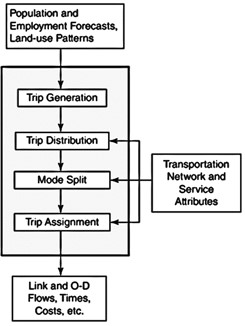
The Four-Step Model (FSM) is comprised of four consecutive steps, each addressing a specific question, ultimately contributing to an enhanced comprehension of travel demand. The questions are:

• Trip generation (Chapter 10) – How many total trips are estimated? What is the demand (total trips)?
• Trip distribution (Chapter 11) – Where are the trip destinations? What are the destinations of the trips?
• Modal split (Chapter 12) – What modes are used to complete those trips?
• Trip assignment (Chapter 13): What routes will be selected to complete the trips? (Meyer, 2016).

Figure 10.1 shows how the model is structured. It shows what kinds of data we provide as input for the model, and what steps we take to generate outputs.

Key Concepts

Link-diverted trips: Trips produced as a result of congestion near the generator and require a diversion; new traffic will be added to the streets adjacent to the site. In other words, these are trips with multiple destinations within one area and do not require road access between destinations.

Diverted trips:  Travel changes in time and route are known as diverted trips. For example, when a trip is diverted or re-routed from the original travel path due to the traffic on nearby roadways, new traffic on surrounding streets results, but the trip attraction remains the same.

Pass-by trips (see below) do not include link-diverted trips.

Pass-by trips: This type of trip is described as a trip for which the destination is not a final but a stop along the way by using the connecting roads. Passing-by traffic volume in a zone depends on the type and size of development or available activities.  A gas station with higher prices near an employment center may receive many pass-by trips for gas compared to other gas stations (Where up to 50 % of all trips to a service station are travelers passing by rather than people who made a special trip to the gas station)

A gas station located in close proximity to an employment center and charging higher prices might experience a higher number of pass-by trips for gas, in contrast to other gas stations. It is observed that up to 50% of all trips to a service station are by travelers passing by, rather than individuals specifically making a deliberate trip to that gas station.  (Meyer, 2016).

Traditional FSM Zonal Analysis   : After inputting the required data for the model, FSM calculates the number of trips generated by or attracted to each zone using the primary input using data from travel surveys from census data. While one limitation of the trip generation model is reduced accuracy due to aggregated data, the model offers a straightforward and easily accessible set of data requirements. Typically, by utilizing basic socio-economic information like population, job figures, vehicle availability, income, and similar metrics, one can calculate trip generation and distribution.

 Activity-based Analysis: There are also other (newer) methods for travel demand modeling in which individual trips are modeled based on individuals’ behaviors and activities in a disaggregated manner. The methods that use activity-based models can estimate travel demand based on a basic premise—the demand to accomplish personal activities during the day (for example, work, school, personal business, and so forth) produces a demand for travel that is often connected (Glickman et al., 2015). However, activity-based models have extensive data requirements as individuals, rather than traffic analysis zones, are the unit of analysis. Detailed information on each individual’s daily activity and socioeconomic information is needed.

Travel diaries (tours) are one source of such information (Ettema et al., 1996; Malayath & Verma, 2013). Because of travel demand modeling, additional information can be learned about the study area. For example, the detailed data may reveal information about areas with or without minimum accessibility, underserved populations, transportation inequity, or congested corridors (Park et al., 2020).

Several scholars have compared the two models – traditional zonal models and activity-based models – to assess factors such as forecasting ability, accuracy, and policy sensitivity. Despite initial expectations, the findings from some studies show no improvement in the accuracy of activity-based models over traditional models (Ferdous et al., 2011). However, considering the complexity of decision-making, activity-based models can be used to minimize the unrealistic assumptions and aggregation bias inherent in FSM models. Still, the applicability and accuracy of activity-based models should be independently assessed for each context analysis to determine which is the most effective approach.

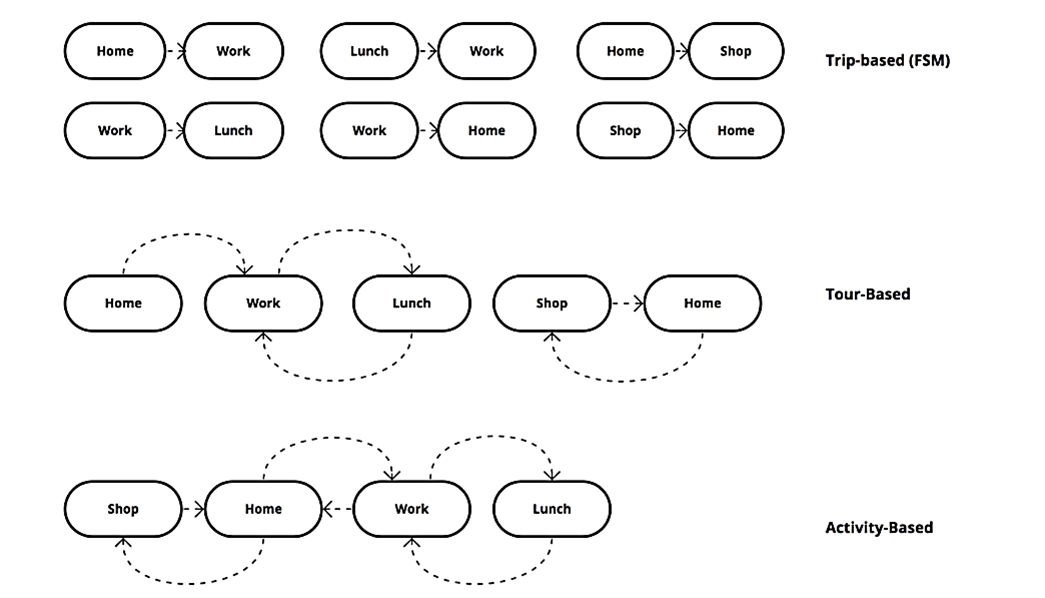
In transportation analysis, trips are typically classified based on the origin (O)and destination (D) location. As mentioned in previous sections, for a more accurate and better estimation of trip generation results, it would be better to identify a wide range of trip categories and have disaggregate results by trip purposes. The following lists typical trip classifications:

• Home-based work (HBW) : If one of the trip origins is home and the destination is the workplace, then we can define the trip purpose as home-based work (HBW). These trips usually happen in the morning (to work) and in the evening (from work to home).
• Home-based non-work (HBNW) : If from the two ends of the trips, one is home and the other one is not workplace, the trip purpose is home-based-non-work (HBNW). Sometimes this trip purpose is called home-se is called home-based other ( HBO ). Examples of these are going to services like a restaurant or hospital.
• Non-home-based (NHB) : If neither the origin nor the destination is home, we can classify the trip as a non-home-based (NHB) purpose. One typical example is a lunch break trip from the workplace to a shopping mall.

While the above categories include only one origin and one destination, most individual trips are more complex due to chaining different trips into one tour. For instance, a person may stop for coffee or drop their child at daycare on the way to work, leave on lunch break for shopping, and then pick up their child from daycare on the way home. A tour is a continuous chain of trips an individual takes daily to complete their chores, which activity-based models can simulate (Ben-Akiva & Bowman, 1998).  Figure 10.2 illustrates the different trip purposes and differences between FSM and activity-based models in trip classification.

It is important to note that home-based trips can be work, school, shopping, recreational, and others. While the first two are usually mandatory and made daily, the rest are less regular or discretionary.

Trips can also be classified based on the time of day that they are generated or attracted, as traffic volumes on various corridors vary throughout the day. Essentially, the proportion of different trip purposes in the total trips is more pronounced during specific times of the day, usually categorized as peak and off-peak hours (Alkaissi, 2021).

Lastly, another factor to consider is the socio-economic characteristics and behaviors of the trip makers. An understanding of these factors is crucial for classifying trips, as some possess significant influence on travel behavior (Giuliano, 2003; Jahanshahi et al., 2009; Mauch & Taylor, 1997), such as, income level, car ownership, and household size.

Trip generation

Recall from the previous chapter, a comprehensive analysis of travel demand should include trip generation and attractions for different zones. These values should be balanced to produce an equal number of trips. In general, trip generation helps predict the number of trips for different purposes generated by and attracted to every zone in a study area.

Additionally, the number of trip ends – the total number of trips entering and leaving a specific land use or site over a designated period – can be calculated in the trip generation step (New Jersey Transit, 1994). Despite recent trends for remote work, most people do not live and work in the same area. Daily round trips to work or shopping centers originate from different locations. In this regard, the distribution of activities, like job centers, can help us to understand daily travel patterns (Wang & Hofe, 2020).

After generating an overview of the distribution of activities and land uses, we must identify the factors or conditions affectingtripgeneration. Over the years, studieshaveexaminedfactorsthatarenow accepted as standard:income,autoownership,familysize,ordensity(Ewingetal.,1996;Sharpeetal.,1958).Using a zonal level analysis, population, number of jobs, and availability of modes can affect trip generation (Wang&Hofe,2020).Similarly,thetypeandsizeofretailstores canalsoaffectthenumberoftrips.

Additionally, the predominant travel mode chosen by the population for their daily trips is a vital factor to consider. Because of the interconnectedness of land use and transportation, the primary mode influences the distribution of services, employment centers, and the overall structure and boundaries of the city. In summary, the type and intensity of land use in combination with transportation mode play crucial roles in trip generation.

The table below shows 5 hypothetical cities where the predominant mode of transportation is different for each case. According to the speed of each mode, the extent to which activities are dispersed, determines the size of the city. For instance, a city where rail is the frequent mode of transportation, the speed (21 mph) and travel time (43 mins), the catchment (distance) would be 12 miles. Using this distance as a radius, we can estimate the size of the city.

Table 10.1 Hypothetical cities with different transportation modes

According to the discussion here, the following categories can be identified as contributors to trip generation (McNally, 2007).

• Land-use types
• Land-use Intensity
• Location/accessibility
• Travel time
• Travel mode (transit, auto, walking …)
• Households’ income level
• Auto ownership rate
• Workers per household

Trip Generation Calibration

Traffic Analysis Zones (TAZs) connected by transportation networks and facilities are used to model the study area. TAZs are the smallest units of analysis in FSM. They are typically bounded by transportation networks or natural boundaries such as rivers.

Prior to estimating trip generators and attractions, calibrate the model as follows:

• Determine the regional population and the employment rate for the forecasting year to estimate the total number of interactions and possible future patterns.
• Allocate population and economic activities to each TAZ to prepare the study area for the modeling framework.
• Specify the significant variables and a proper method for creating the travel demand model (trip generation step). This step can be called model specification.

Calibration is an essential process in travel demand modeling. It involves collecting actual traffic flow data and calculating model parameters to verify the accuracy of the model for a specific region. The purpose of calibration is to match predicted outcomes with observed data, ensuring that model results are reliable and trustworthy (Wang & Hofe, 2020).

FSM MODELING UNITS

As discussed previously, the unit of analysis used for the model varies by model type.  The unit of analysis is important as it guides data collection. Traditional zonal analysis, like FSM, typically uses TAZs.  Activity-based models typically use data at the level of the individual person or household. There are three general methods for trip generation estimations:

1.     Growth factor model,

2.     regression methods,

3.     cross-classification models (tables),

4.     and rates based on activity units (ITE).

Generally, the trip generation step requires two types of data – household-based and zonal-based. Household-based data is more suitable for cross-classification analysis , and zonal-based data is more applicable for regression method analysis (the following sections will discuss these methods).

The third method is based on rates by which each land use type generates trips. The very general process for this method is identifying land use types, estimating trip generation according to ITE manuals, calculate total generation, and finally modifying based on specific characteristics such as proximity or location of land use. In this chapter, we do not wish to illustrate the third model, instead we focus on regression and cross-classification models since they are more data-oriented methods, more realistic and more frequently used in real-world.

The zonal analysis consists of areas divided into smaller units (zones), from which an estimate of trips generated in each zone is obtained (aggregate model). Household-based analysis decomposes zones into smaller units based on households with similar characteristics. In transportation travel demand modeling, we estimate zonal trips for various purposes, such as work, school, shopping, and social or recreational trips. As said, a zone is an area with homogeneous characteristics of land use, population, income, vehicle ownership, and the same access path outside of the zone.

In many cases, however, sufficient data at this resolution is unavailable (available at Census Tracts, Blocks, and Block Groups). In these conditions, the modeler should assess if the lower-resolution data is sufficient for their purpose. If not, using appropriate GIS-based data conversion methods, the data from a higher level (such as Census Tract) can be migrated to lower-level units (such as TAZ).

GROWTH FACTOR MODELING

A straightforward approach for estimating future trip generation volumes is to translate trends from the past into the future based on a linear growth trend of effective factors such as population or income. This method projects past data into the future by assuming a constant growth rate between two historical points. We can use this method when trip production and attraction in the base year are available, but the cost function (like travel time) is not. While this method is commonly used, it is important to note that it is insensitive to the distance between zones, which affects the estimated future data (Meyer, 2016).

In this model, the future number of trips equals the number of current trips times the growth factor.

Equation below is the method’s mathematical format:

T i is the number of trips in the zone in the forecasting year

t i is the current number of trips in that zone

f i is a growth factor

The growth factor itself consists of a number of explanatory variables that we acknowledge have impact on trip generation such as population, income (I), and ownership (V). To calculate a single growth factor with all these variables, the below equation is useful:

P i d is the population in the design year

P i c is the population in the current year

I i d is the income level in the design year

I i c is the income level in the current year

V i d is the vehicle ownership rate in the design year

V i c is the vehicle ownership rate in the current year

In a small neighborhood, 630 households reside, out of which 300 households have cars and 330 are without cars. Assuming population and income remain constant, and all households have one car in the forecasting year, calculate the total trips generated in the forecasting year and the growth factor (trip generation rate for 1-car: 2.8; 0-car:1.1). Assume that a zone has 275 households with cars and 275 without cars, and the average trip generation rates for the two groups are 5.0 and 2.5 trips per day.

Assuming all households will have a car in the future, find the growth factor and the future generated trips from that zone, keeping population and income constant.

• Current trip rate ti=300 × 2.8 + 330 × 1.1 = ? (Trips/day)
• Growth factor Fi=Vdi/Vc =630/300= ?
• Number of future trips Ti = Fiti = 2.1 × 1203 = ? (Trips / day)

Regression Analysis

Regression analysis begins with the classification of populations or zones using the socio-economic data of different groups (like low-income, middle-income, and high-income households). Trip generation can be calculated for each category and the total generated trips by each socio-economic group such as income groups and auto ownership groups using linear regression modeling. The reason for disaggregating different trip making groups is that as we discussed, travel behavior can significantly vary based on income, vehicle availability and other capabilities. Thus, in order to generate accurate trip generations using linear models such as OLS (Ordinary Least Squares) regression, we have to develop different models with different trip making rates and multipliers for different groups. This classification is also employed in cross-classification models, which is discussed next. While the initial process for regression analysis is similar to cross-classification models, one should not confuse the two methods, as the regression models attempts to fit the data to a linear model to estimate trip generation, while cross-classification disaggregates the study area based on characteristics using curves and then attributes trips to each group without building predictive models.

Alternatively, the number of total trips attracted to each zone would be determined using regression analysis on employment data and land-use attraction rates. The coefficients for the prediction model in linear regression analysis can be derived. The prediction model has a zone’s trip production or attraction as a dependent variable, and independent variables are socio-economic data aggregated by zone. Below, we illustrate a general formula for the regression type analysis:

Trip Production= f (median family income, residential density, mean number of automobiles per household)

The estimation method in this regression analysis is OLS (Ordinary Least Squares). After zonal variable data for the entire study area are collected, linear regression analysis is applied to derive the coefficients for the prediction model. A major shortcoming associated with this model is that aggregate data may not reflect the precise effect of data on trip production. For instance, individuals in two zones with an identical vehicle ownership rate may have very different access levels to private cars, thus having different trip productions. The cross-classification model described in the next section helps address this limitation (McNally, 2007).

Equation below shows the typical mathematical format of the trip generation regression model:

where X i is the independent variable and a i is the associated coefficient.

In a residential zone, trip production is assumed to be explained by the vehicle ownership rate of households. For each household type, the trip-making rates are shown in Table 10.2). Using this information, derive a fitted line. Table 10.2 documents 12 data points. Each corresponds to one family and the number of trips per day. For instance, for a 1-vehicle family, we have (1,1) (1,3), and (1,4).

Table 10.2 Sample vehicle ownership data for trip generation

The linear equation will have the form: y = bx + a. Where: y is the trip rate, and x is the household vehicle ownership, and a and b are the coefficients. For a best fit, b is given by the equation:

Based on the input table, we have:

Σx = 3 × 1 + 3 × 1 + 3 × 3 + 3 × 3 = 24 Σx2 = 3 × (1 2 ) + 3 × (2 2 ) + 3 × (3 2 ) + 3 × (4 2 ) = 90 Σy = 8 + 14 + 21 + 28 = 71 Σxy = 1 × 1 + 1 × 1 + 1 × 3 + 1 × 3 + 2 × 2 + 2 × 3 + 2 × 4 + 2 × 5 + 3 × 5 + 3 × 4 + 3 × 5 + 3 × 7 + 4 × 7 + 4 × 5 + 4 × 8 + 4 × 8 = 211

y‾ = 71/12 = 5.91 x‾ = 30/12 = 2.5 b = (nΣxy − ΣxΣy)/[(nΣx 2 − (Σx) 2 ] =((16 × 211) − (24 × 71))/((16 × 90) − (24) 2 ) = 1.93 a = y‾ − b x‾ = 17.75 – 1.93 × 2.5 = 12.925 y= 1.93X + 12.925

Cross Classification Models

This type of model estimates trip generation by classifying households into zones based on similarities in socio-economic attributes such as income level or auto ownership rate. Since the estimated values are separate for each group or category of households, this model aligns with our presumption that households with similar characteristics are likely to have similar travel patterns (Mathew & Rao, 2006). The first step in this approach is to disaggregate the data based on household characteristics and then calculate trip generations for each class. Aggregate all calculated rates together in the final step to generate total zonal trip generations. Typically, there are three to four variables for household classification, and each variable includes a few discrete categories. This model’s standard variables or attributes are income categories, auto ownership, trip rate/auto, and trip purpose.

The cross-classification method involves grouping households based on different characteristics such as income and family size. For each group, the trip generation rate can be calculated by dividing the total number of trips made by families in that group by the total number of households in that group within each zone (Aloc & Amar, 2013).

The following are some of the advantages of the cross-classification model:

• Groupings are independent of the TAZ system of the study area.
• No need to assume linearity as it disaggregates the data.
• It can be used for modal split.
• It is simple to run and understand. Furthermore, some of the model’s disadvantages are:
• It does not permit extrapolation beyond its calibration strata.
• No measure of goodness of fit is identifiable.
• It requires large sample sizes (25 households per cell); otherwise, cell values will vary.

After exploring the general definitions and features of the cross-classification model for trip generation estimations, we present a specific example and show how to perform each model step in detail.

Suppose there is a TAZ that contains 500 households, and the average income for this TAZ is

$35000. We are to develop the family of cross-classification curves and determine the number of trips produced by purpose. The low, medium, and high income are $15,000, $25,000, and $55,000, respectively (Note: this data is extracted from 1990 and is therefore out of date. Current rates for income categories may be higher.) (Adapted from: NHI, 2005). For the first step, we should develop the family of cross-class curves for the income levels and find the number of households in each income category.

If we divide the households by six income ranges, we have the table below, derived from the survey.

Based on this table, we can plot the curves in the following format:

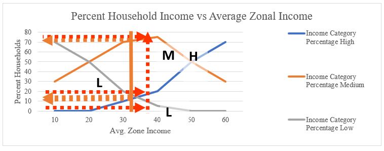
If you look at the vertical line on the $40,000 income level, you can find that the intersection of this line with three income range categories shows the percentage of households in that range. Thus, to find the number of total households in each group we have to find the intersection of the curves with average income level ($35,000). In the above plot, the orange line shows these three values, and the table below can be generated according to that:

2. In the second step, after deriving the number of households in each income category, we follow the same procedure for other variables: vehicle ownership. In other words, now we find trips per household in each auto ownership/income group “class.” Again, from the survey, we have the following table, and we can generate the plot of the curves according to that:

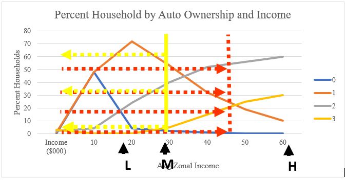
Like the previous step, the intersection of four auto ownership curves with low, medium, and high-income level lines determine the share of each auto ownership rate in each income level group:

3. After calculating the number of households in each income level category and auto ownership rate, the next step in the trip generation estimation procedure is to find the number of trips per household based on income level and auto ownership rate. The table below shows the trip generation rate for different income levels:

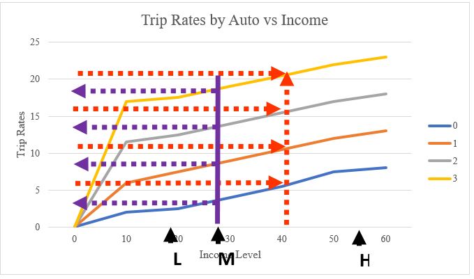
In Figure 10.3, the meeting point of three income levels and auto ownership status with trip rates yields us the following table:

4. In the fourth step, we must incorporate the trip purpose into the model. To that end, we have trip purposes ratios based on income level from the survey. Like the previous steps, we plot the table on a graph to visualize the curves and find the intersection points of the curves with our three low, medium, and high-income levels:

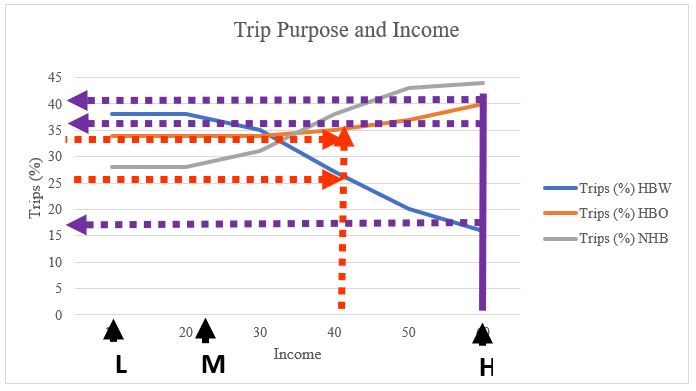
Based on the findings of this plot, we can now generate the table below, in which the percentage of trips by purpose and income level is illustrated:

Now, we have all the information we need for calculating the total number of trips by household income level and trip purpose.5.

5. In the next step, we calculate the total number of households in each income group based on the number of cars they own. Multiplying the number of households in each income group (00) to the percent of families with a certain number of cars (A) will give us the mentioned results.

6. Once we have the total number of households in each group of income based on auto ownership, we multiply the results to the trips rate (B) so that we have the total number of trips for each group.

7. In the next step, we sum the results of the number of trips by the auto ownership number to have the total number of trips for each income group (∑(00xAxB)).

8. Finally, the results from the above table (416, 3474, 1395) will be multiplied by the percentage of trip purposes for each income group in order to estimate the number of trips by trip purposes for each income group. The table below shows these results as the final trip generation results (example adapted from: NHI, 2005).

Cx∑(00xAxB):

Trip Attraction in the Cross-Classification Model

In the previous section, we modeled trips generated from different households and zones, and calculated their total number by purpose. However, in trip generation, trip attractions play a crucial role, along with trip production. To measure the attractiveness of zones, we can use an easy and straightforward method, which is to determine the size of each zone and the land use types within it, such as square feet of floor space or the number of employees. We can then derive trip generation rates for different attractions from surveys. Trip attractions refer to the number of trips that end in one zone. Typically, we express trip generation rates for different attractions in terms of the number of vehicle trips per household or unit area of non-residential land use. For instance, Table 10.13 provides trip attraction rates for residential and some non-residential land uses. The number 0.074 for HBW trips means that each household can attract 0.074 HBW vehicle trips per day. For non-residential land uses, the numbers are also dependent on the type and size of land uses. As shown in Table 10.13, the retail sector is more attractive than the basic sector.

Table 10.13 shows that the retail sector is more attractive than the basic sector.

After collecting the necessary data from surveys or other appropriate sources, a regression analysis can be used to determine the attraction rates for each land-use category. Then, the HBW vehicle trips attracted to a zone are then calculated as:

TA HBW_H = home-based work vehicle trip attractiveness of the zone by households

N hh = number of household in the zone

TAR _R = trip attraction rate by households

In a similar way, the HBW trips attracted by retail are calculated from the size of retail land use and the retail trip attraction rates.

TA HBW_NR = home-based work vehicle trip attractiveness of the zone

A _NR = non-residential land use size in the zone

TAR _NR = trip attraction rate of the non-residential land use

Assume that Table 10-14 is derived from survey data in a hypothetical city and attractiveness of each land use by trip purpose is generated.

Additionally, a new retail center in a part of the city accommodates 370 retail workers and 550 non-retail workers. According to this information, the number of trips attracted to this area can be calculated as:

First, using the information in table 10.14:

HBW: (370 * 1.7) + (550 * 1.8) = 1619

HBO: (370 * 5.4) + (550 * 2.2) = 3208

NHB: (370 * 3.0) + (550 * 1.1) = 1715

Total = 6542trips/day (example adopted from: Alkaissi, 2021)

Balancing Attractions and Productions

After generating trips, the final step is to balance trip production and attraction. Since trip generation is more accurate, and its validity is more reliable compared to trip attraction models, attraction results are usually brought to the scale of trip generation. Balance factors are used to balance Home-Based Work (HBW) trip attraction and production, which is illustrated in the example below.

According to Table 10.15, the total number of trips generated by all three zones is 600. However, the total number of trips attracted to all the zones is 800, which is an unreasonable value. To fix this issue, we use a balancing factor to multiply each cell in the attraction column by (600/800).

When planning NHB (non-home-based) trips, it is important to take an extra step to ensure that the production and attraction outputs are balanced. This means that for all zones and each zone, the total number of trips attracted and generated should be the same. The reason for this is that NHB trips have unknown origins, meaning that the origin information is not available through surveys or census data. Therefore, the most accurate estimate possible is to set the total NHB productions and attractions to be equal.

In this chapter, we introduced and reviewed the first step of travel demand modeling that is developed for estimating trip generation from each neighborhood or zone. We specifically focused on different methods (growth factor, regression, and cross-classification) and provided examples for each method along with an overview of key concepts and factors contributing to trip generation. Today, the ongoing advancements in computational capacity as well as capabilities for real-time data collection appear to be promising in equipping us with more accurate predictions of trip generation. For instance, GPS mobile data can be used to empirically estimate the rate of trip generation, build advanced models (such as machine learning models) to develop highly calibrated and optimized models.

In the next chapter, we learn about trip distribution. It is worth noting here that the trip distribution is completely based on a foundation of attractiveness of various location determined in trip generation step. As we will see, we used gravity-based models to allocate demand to pair of zones in space. In other words, four-step model is a sequential model, in which the accuracy and reliability of the each step depends on model performance in previous steps.

• activity-based model is travel forecasting framework which is based on the principle that travel is derived from demand reflected in activity patterns of individuals.
• Travel diaries (tours) refers to a chain of trips between multiple locations and for different purposes such as home to work to shopping to home.

Land-use Intensity is a measure of the amount of development on a piece of land usually quantified as dwelling per acre.

• Pass-by trips refers to the trips for which the destination is not a final destination but rather an stop along the way by using the connecting roads.
• Diverted link trips are produced from the traffic flow in the adjacent area of the trip generator that needs diversion. This new traffic will be accumulated in the roadways close to the site.

Key Takeaways

In this chapter, we covered:

• What trip generation is and what factors influence trip generation.
• Different approaches for estimating trip generation rates and the data components needed for each.
• The advantages and disadvantages of different methods and assumptions in trip generation.
• How to perform a trip generation estimation manually using input data.

Prep/quiz/assessments

• List all the factors that affect trip generation. What approaches can help incorporate these factors?
• What are the different categories of trip purposes? How do newer (activity-based models) models differ from traditional models (FSM) based on trip purposes?
• What are the data requirements for the growth factor model, and what shortcomings does this method have?
• Why should trip productions’ and attractions’ total be equal, and how do we address a mismatch?

Alkaissi, Z. (2021). Trip generation model. In Advanced Transportation Planning, Lecture, 4. Mustansiriya University   https://uomustansiriyah.edu.iq/media/lectures/5/5_2021_05_17!10_34_51_PM.pdf

Aloc, D. S., & Amar, J. A. C. (2013). Trip generation modelling of Lipa City . Seminar and research methods in civil engineering research program, University of Philippines Diliman. doi: 10.13140/2.1.2171.7126.

Ben-Akiva, M.E., Bowman, J.L. (1998). Activity based travel demand model systems. In: P. Marcotte, S. Nguyen, S. (eds) Equilibrium and advanced transportation modelling. Centre for Research on Transportation . Springer, Boston, MA. Kluwer Academic Publishers, pp. 27–46.  https://doi.org/10.1007/978-1-4615-5757-9_2

Ettema, D., Borgers, A., & Timmermans, H. (1996). SMASH (Simulation model of activity scheduling heuristics): Some simulations. Transportation Research Record , 1551 (1), 88–94. https://doi.org/10.1177/0361198196155100112

Ewing, R., DeAnna, M., & Li, S.-C. (1996). Land use impacts on trip generation rates. Transportation Research Record , 1518 (1), 1–6. https://doi.org/10.1177/0361198196151800101

Giuliano, G. (2003). Travel, location and race/ethnicity. Transportation Research Part A: Policy and Practice , 37 (4), 351–372. https://doi.org/10.1016/S0965-8564(02)00020-4

Glickman, I., Ishaq, R., Katoshevski-Cavari, R., & Shiftan, Y. (2015). Integrating activity-based travel-demand models with land-use and other long-term lifestyle decisions. Journal of Transport and Land Use , 8 (3), 71–93. https://doi.org/10.5198/jtlu.2015.658

ITE, I. of T. E. (2017). Trip generation manual . ITE Journal. ISSN 0162-8178. 91(10)

Jahanshahi, K., Williams, I., & Hao, X. (2009). Understanding travel behaviour and factors affecting trip rates. In  European Transport Conference, Netherlands (Vol. 2009). https://www.researchgate.net/profile/Kaveh Jahanshahi/publication/281464452_Understanding_Travel_Behaviour_and_Factors_Affecting_Trip_Rates/links/57286bc808ae262228b5e362/Understanding-Travel-Behaviour-and-Factors-Affecting-Trip-Rates.pdf

Malayath, M., & Verma, A. (2013). Activity based travel demand models as a tool for evaluating sustainable transportation policies. Research in Transportation Economics , 38 (1), 45–66. https://doi.org/10.1016/j.retrec.2012.05.010

Mathew, T. V., & Rao, K. K. (2006). Introduction to transportation engineering. Civil Engineering–Transportation Engineering. IIT Bombay, NPTEL ONLINE, Http://Www. Cdeep. Iitb. Ac. in/Nptel/Civil% 20Engineering .

Mauch, M., & Taylor, B. D. (1997). Gender, race, and travel behavior: Analysis of household-serving travel and commuting in San Francisco bay area. Transportation Research Record , 1607 (1), 147–153.

McNally, M. G. (2007). The four step model. In D. A. Hensher, & K. J. Button (Eds.), Handbook of transport modelling , Volume1 (pp.35–53). Bingley, UK: Emerald Publishing. http://worldcat.org/isbn/0080435947

Meyer, M. D., (2016). Transportation planning handbook . John Wiley & Sons: Hoboken, NJ, USA, 2016.

New Jersey Transit, N. (1994). Planning for transit-friendly land use: A handbook for New Jersey communities . NJ Transit, Trenton, NJ.

NHI. (2005). Introduction to Urban Travel Demand Forecasting . In National Highway Administration (Ed.), Introduction to Urban Travel Demand Forecasting. American University. . National Highway Institute : Search for Courses (dot.gov)

Park, K., Sabouri, S., Lyons, T., Tian, G., & Ewing, R. (2020). Intrazonal or interzonal? Improving intrazonal travel forecast in a four-step travel demand model. Transportation , 47 (5), 2087–2108. https://doi.org/10.3141/1607-20

Sharpe, G. B., Hansen, W. G., & Hamner, L. B. (1958). Factors affecting trip generation of residential land-use areas . Highway Research Board Bulletin, 203 . http://onlinepubs.trb.org/Onlinepubs/hrbbulletin/203/203-002.pdf

Wang, X., & Vom Hofe, R. (2020). Selected methods of planning analysis (2nd ed. 2020 edition). Springer. Springer Nature. https://doi.org/10.1007/978-981-15-2826-2

Whitney, V. (2019, September, 29). Activity & Trip Based Travel Models. Medium . https://medium.com/data-mining-the-city/activity-trip-based-travel-models-e4833571570

Cross-classification is a method for trip production estimation that disaggregates trip rates in an extended format for different categories of trips like home-based trips or non-home-based trips and different attributes of households such as car ownership or income.

Transportation Land-Use Modeling & Policy Copyright © by Mavs Open Press. All Rights Reserved.

Share This Book

Don't miss tomorrow's smart cities industry news

Let Smart Cities Dive's free newsletter keep you informed, straight from your inbox.

At Last! Open Source Trip Generation Data for Transport Planning

We have long known in the transportation planning community that the use of trip generation for local area review, and the Institute of Transportation Engineers (ITE)'s procedure for estimating trip generation is broken in any number of ways. Shoup's Truth in Transportation Planning is a classic critique of the problems.

[Trip generation is the first step in the conventional four-step transportation forecasting process (followed by trip distribution, mode choice, and route assignment), widely used for forecasting travel demands. It predicts the number of trips originating in or destined for a particular traffic analysis zone.]

While we could (and perhaps should) through the whole kit and caboodle into recycling, in practice trip generation methods will be with us decades from now (even as traditional work, shopping and driving disappear). So there is a small academic movement to make the methods better. The most recent issue of JTLU 8(1) has a special section on Trip Generation, including several papers about how to adjust and improve ITE's Trip Generation methods based on better data.

Part of the problem is that ITE is functionally a for-profit organization, and makes bank on selling the Trip Generation Manual and associated software (recognizing the fact that use of ITE Trip Generation rates is ensconced in law and regulation).

What has long been needed is an open source database of trip generation studies so that better fits to actual site conditions can be used in analysis. I recall in my youth some engineers in Montgomery County, Maryland trying to set something up, but this was well before the world wide web made that easy.

Fortunately that day is upon us. Mike Spack and company have set up TripGeneration.org , which is populated with open access trip generation studies (licensed under a Creative Commons license), and for which they hope to grow the data set.

This set is professionally collected and currently holds 2500+ hours of data. Signing up gets you sent the current Trip Generation Data Spreadsheet.

This is new, and I assume as it grows the data will get better and better, as will the methods for inputting and extracting data. Kudos to Mike, Nate, and others at Spack Consulting for getting this going. I look forward to seeing where this goes, as Big Data and new sensors make data collection increasingly ubiquitous.

Related posts:

• Smart Growth and Trip Prediction
• Does smart growth actually reduce congestion?
• STUDY: City Living = As Much CO2 As Rural Life
• It's Definitely Time to Rethink the Parking Lot
• Is This the First Post-Car-Dependent Generation in America?
• Why Public Transport Needs to Work for Women, Too
• San Francisco's Director of Transportation Planning on the Importance of Piloting Integrated Infrastructure
• Pragmatic Planning for a Sustainable Transportation System
• Integrating Health Benefits into Transport Planning and Policy

An official website of the United States government

Here’s how you know

Official websites use .gov A .gov website belongs to an official government organization in the United States.

Secure .gov websites use HTTPS A lock ( Lock A locked padlock ) or https:// means you’ve safely connected to the .gov website. Share sensitive information only on official, secure websites.

JavaScript appears to be disabled on this computer. Please click here to see any active alerts .

Mixed-Use Trip Generation Model

Neighborhoods that mix land uses and make walking safe and convenient allow residents and workers to drive significantly less, thereby reducing traffic and realizing other benefits.

To help give communities better tools to analyze new development, EPA, in cooperation with the Institute of Transportation Engineers (ITE), worked with leading researchers and practitioners to develop new data and methods to estimate the trip-generation impacts of mixed-use developments. 

Download the  Mixed-Use Trip Generation Tool .

On this page:

Purpose of the Tool

• How the Tool was Created

Additional Resources

Trip generation analysis, the technical methodology to estimate how much traffic a new development will create, have been standardized by ITE and are used by traffic engineers across the country.

However, these methods are generally based on data collected from single-use, automobile-dependent, suburban sites, and therefore they do not adequately account for the effects of compact development, mix of uses, site design, walkability, transit, and regional accessibility – key elements of smart growth strategies and of a sustainable community.

To address this challenge, EPA created a spreadsheet tool that makes it easy for local stakeholders to estimate the internal capture of trips generated by a new mixed-use development. 

The spreadsheet estimates vehicle trips generated by a new mixed-use development in peak periods and for an entire day. The method also predicts trips by walking and transit and estimates the daily vehicle miles of travel associated with the development. 

How the Tool Was Created

In order to create the tool, EPA analyzed six metropolitan regions, merging data from household travel surveys, GIS databases, and other sources to create consistent land use and travel measures. The tool requires information about the development site and its surrounding area, including geographic, demographic, and land use characteristics.

It includes default national parameters for trip generation, but allows the use of local values if available. An associated report, available upon request, describes the research basis for the method and the data used to calibrate and validate it. 

This method was used in several regions in California, Washington, and New Mexico, and the Virginia Department of Transportation adopted it as a statewide standard for determining the traffic impacts of urban mixed-use developments.

The following resources give more information on development, testing, and use of the method and tool:

• Traffic Generated by Mixed-Use Developments – A Six-Region Study Using Consistent Built Environmental Measures , Ewing et al., ASCE Journal of Urban Planning and Development , 2011. This peer-reviewed article describes the analytic basis for the models, database development, and reports on validation tests. (Fee or subscription required.)
• Mixed-Use Development Trip Generation , Fehr & Peers. This website, by the firm that led development of the tool for EPA, describes the tool and reports on the statistical validation of the models.
• Smart Growth Trip Generation and Parking Study , San Diego Association of Governments (SANDAG), 2010. SANDAG approved the method for use regionwide following comparison to local sites and review by local staff. This web page provides details on its review and implementation.

The following resources describe standard trip generation methods and other efforts to better understand the impacts of mixed-use developments and related smart growth strategies:

• Trip and Parking Generation Technical Resources , Institute of Transportation Engineers. Links to trip generation publications and other resources.
• Enhancing Internal Trip Capture Estimation for Mixed-Use Developments ,  National Cooperative Highway Research Program Report 684, 2011. This method, similar in scope to the EPA method described above, estimates peak-period internal capture rates for mixed-use developments for use in standard ITE trip generation applications.
• Effects of TOD on Housing, Parking, and Travel , Transit Cooperative Research Program Report 128, 2008. This report gives insight into the characteristics of residents of transit-oriented development, including their trip generation rates. 
• Smart Growth Home
• About Smart Growth
• Technical Assistance
• Examples of Smart Growth
• Publications
• Webinars, Videos, and Podcasts
• Smart Growth in Your Community

Jump to navigation

National Institute for Transportation and Communities

Search form.

• Latest News
• Media Coverage
• Join Our Mailing List
• Final Reports
• NITC Researchers
• Requirements and Forms
• Researcher Login
• Curriculum: K-12 and University
• A decade of NITC research
• Transportation and Land Use
• Multimodal Data and Modeling
• Walking and Biking
• New Mobility and Technology
• Equitable Mobility
• Transportation Resiliency
• Upcoming Events
• Annual Summit
• K-12 Programs
• Past Events
• Student Spotlights
• Student of the Year
• Dissertation Fellowships
• Student Groups

Moving From Cars To People: A Comic About Transportation and Land Use

A new transportation comic, " Moving From Cars To People (PDF), " offers a succinct and fun introduction to a complicated topic: namely, how the built environment in the United States came to be designed for cars and what we can do about it.

Want a physical copy? Here are a few ways to get one:

• Request a free copy from our limited print run (first come, first served)
• Order a copy for just the cost of printing & shipping;
• Print one yourself at any local printer, with our high-res print-...

Polycentric Development: How the Built Environment Affects Travel Behavior

NITC research led by Reid Ewing of the University of Utah, examining impacts that the built environment and development patterns have on transportation, has produced a number of journal articles in the past year. Three 2021 articles highlighted below each focus on different aspects of the body of work, which revolves around polycentric development and trip generation.

A May 2021 article in the Journal of Transport Geography  estimated a vehicle ownership model that contributes to our understanding of vehicle ownership and improves the accuracy of travel demand forecasts. " The built environment and vehicle ownership modeling: Evidence from 32 diverse regions in the U.S. ," authored by Sadegh Sabouri, Guang Tian, Reid Ewing, Keunhyun Park and William Greene, draws on findings from the NITC project Key Enhancements to the WFRC/MAG Four-Step Travel Demand Model . 

Two main outcomes of this paper are:

• The number of vehicles owned by a household increases with socio-demographic variables and decreases with almost all of the built environmental variables. For the urban planning and design practices, this finding suggests that car shedding occurs as built environments become more dense, mixed, connected,...

New Travel Demand Modeling for Our Evolving Mobility Landscape

• Download the Final Report (PDF)
• Download the Project Brief (PDF)
• Watch the February 2020 webinar

Conventional four-step travel demand modeling is overdue for a major update. The latest NITC report from the University of Utah offers planners better predictive accuracy through an improved model, allowing for much greater sensitivity to new variables that affect travel behavior. Specifically, it accounts for varying rates of vehicle ownership , intrazonal travel , and multimodal mode...

The Advantages and Limitations of Land Use Codes for Multifamily Housing Trip Generation

• See the big picture: Read about the ongoing work

Many cities are reconsidering their reliance on ITE's Trip Generation Manual , now in its 10th edition. 

Kelly Clifton, TREC researcher and associate dean for research of Portland State University's Maseeh College of Engineering & Computer Science, is one of the people leading the charge to identify better, more nuanced ways to anticipate transportation demand; especially person (non-car) trips. In an extended series of TREC projects, Clifton and...

Context-Specific Modeling Supports Strategic, Multimodal Investments

In recent decades, cities have become increasingly motivated to invest in infrastructure that supports multimodal options like walking, biking and public transit. Trip generation, the first step in conventional four-step forecasting models, is a central figure in determining how those investments are made.

However, when considering pedestrian and bicycling travel, the current practice is usually to either leave those trips out of the model altogether, or to simply present them as a mode choice option that is not analyzed further. In short, they’re car-centric.

Without reliable trip generation rates for anyone but drivers, an accurate transportation impact is difficult to predict. Certain land uses will draw far more walkers, cyclists and transit riders than drivers. Cities...

City uses TREC research to better set development fees

The city of Portland is using research and expertise from TREC researchers to change how it calculates fees for new development. Developers pay the fees, called transportation system development charges, to offset some of the costs of providing transportation infrastructure.   The foundation for those fees has been cars: that is, how many car trips a development will generate. In December, the Portland City Council voted to instead use “person trips” as the basis for those fees.   Researchers Kelly Clifton and Kristina Currans have assembled an impressive portfolio of research projects on trip generation. Their research caught the attention of city officials, who brought Clifton and Currans in as consultants to help them rethink the way they assess new fees for development.   Their work found a receptive audience of practitioners at TREC’s flagship conference, the Transportation and Communities Summit , last fall. Clifton and Currans held a workshop on improving trip generation methods to better represent the mix of modes found in livable communities. That led to a collaboration with transportation consultants...

Researchers expand trip generation to include people walking, biking and riding transit

A new NITC report offers a multimodal framework for transportation impact analysis – a welcome tool for professionals in many cities seeking more detailed data about non-drivers.

Improving Trip Generation Methods for Livable Communities , a research project headed by Kelly Clifton of Portland State University and Nico Larco of the University of Oregon, is the latest effort in an ongoing collaboration to create more open sourced, widely available data about non-motorized road users.

Over the last decades, cities have become more invested in fostering the conditions to support walking, biking and public transit.

The land development process presents a unique challenge.

Prior to a zoning change or new development, someone has to determine what its impact on the transportation system will be, and whether upgrades will be necessary to accommodate travelers to the new destination. Trip generation is the first step in the conventional transportation forecasting process.

Current trip generation methods used by engineers across the country tend to focus on motorized modes.

Without reliable trip generation rates for anyone but drivers, the transportation impact is difficult to predict. Certain land uses will draw far more walkers,...

OTREC research looks into contextual influences on trip generation

News from TRB: Making trip-generation models work for urban transportation

Planners looking to develop an dense mix of urban land uses often face a dilemma: they’re using trip-generation models that undercount the very trips on bicycle and foot that the planners encourage while paving the way for more driving.

Portland State University Associate Professor Kelly Clifton dove into the topic Monday, presenting a paper at the Transportation Research Board annual meeting in Washington D.C. Kristina Currans of PSU, April Cutter of Metro, and Robert Schneider of the University of California Berkeley are coauthors.

Clifton and other panelists agreed that the Institute of Transportation Engineers’ trip generation rates don’t adequately reflect actual trips in an urban area with multiple land uses and transportation modes. They differed on the remedy, however.

Presenting another paper, Associate Professor Kevan Shafizadeh of California State University Sacramento, evaluated and tested several complex methods, finding that none truly suits smart-growth development projects. However, Shafizadeh and his team found that every method tested does a better job at predicting the number of trips generated than the ITE rates.

We need to predict trips better, Clifton said, but perhaps a simpler solution exists. She acknowledged Shafizadeh’s conclusions that each alternative also had deficiencies in certain applications, and suggested that the ITE rates could be tweaked instead of scrapped entirely.

“It’s a Band-Aid to temporarily adjust...

Empty Spaces webinar confronts parking at transit-oriented developments

Smart Growth America hosted a webinar Jan. 31 on NITC research finding that standard guidelines lead to a drastic oversupply of parking at transit-oriented developments. That restricts the supply of housing , office and retail space while driving up the price.

The webinar marks the release of Smart Growth America's lay summary of the NITC report, called "Empty Spaces," which will be available to webinar attendees.

Watch the recorded webinar here .

The research, led by Reid Ewing of the University of Utah, is one of the first comprehensive data-driven reports to estimate peak parking and vehicle trip generation rates for transit-oriented development projects, as well as one of the first to estimate travel mode shares for TODs. Ewing analyzed data on actual parking usage and total trip generation near five transit stations: Redmond, Washington; Rhode Island Row in Washington, D.C.; Fruitvale Village in Oakland, California; Englewood, Colorado; and Wilshire/Vermont in Los...

• Forecasting

7  comments

Traffic Impact Study Improvements: Part 5 – When is a Trip Not a Trip?

By   Mike Spack

October 27, 2015

Guest Post by Bryant Ficek, PE, PTOE, Vice President at Spack Consulting

Earlier this year, I detailed how our standard process for a Traffic Impact Study has several points of assumptions at best or guesses at worst. This post continues that discussion.  Check out the “ Top 6 Ways to Pick Apart a Traffic Study ” for more on the general topic and expect more posts to follow on this subject.

Trip generation is the process of estimating the amount of traffic a proposed development will have once it is built and operating. Trip distribution is the process by which we take the raw projected traffic for a development (trip generation) and add it to the existing volumes on the transportation network. The step in-between is determining whether all the trip generation will be new to the roadway.

To start with, there are several types of trips as follows (with definition summarized from the Institute of Transportation Engineers or ITE). The figure below illustrates the different types of trips.

• Primary or New.  Traffic with the specific purpose of visiting the site being studied.
• Pass-By.  Traffic already on the way from an origin to a primary trip destination that will make an intermediate stop at the site being studied without a route diversion.
• Diverted. Traffic attracted to the site being studied from adjacent facilities without direct access to the site. A diverted trip example is a through trip on a freeway that diverts to an exit and a development, adding traffic to the local road but removing traffic from the freeway.
• Internal.  Traffic associated with multi-use developments where trips among various land uses can be made on the site being studied without using the major street system. These trips can be made either by walking or by vehicles using internal roadways.

These different trip generation options, combined with so many different types of land uses, leads to virtually limitless possibilities for the amount and type of traffic a particular site could generate on the roadway system. As with our trip distribution column, we initially thought about testing multiple scenarios, which would be relatively easy with today’s software. At least, theoretically. To restate our collective conclusion – While interesting on a pure research level, a thicker actual traffic impact study report covering multiple results leads us down a path no one wants to go.

Furthermore, sub-dividing the raw trip generation into parts is not something that can be quantified into a “one-size fits all” equation. Given the possibilities and the limits of our collective traffic research to date, ITE provides the best procedure to follow. So this article is dedicated to reviewing that procedure, which is spelled out in ITE’s Trip Generation Handbook and Trip Generation Manual, Volume 1 . That step-by-step process is as follows:

• Raw Trip Generation.  Using ITE or other land use information (try tripgeneration.org !), calculate the raw trip generation for the site.
• Pass-By and Diverted Number of Trips. Use either local data or ITE data to determine a percentage of the reduced trip generation that is pass-by or diverted. Similar to the ITE Trip Generation data, both pass-by and diverted trip percentages are available by average rate or an equation for many land uses. Use this percentage to calculate the total pass-by and diverted trips for the site.
• Pass-By and Diverted Trip Patterns. Use the existing traffic to determine how the pass-by and diverted trips will access the site.
• Pass-By and Diverted Trip Volume Adjustment. Apply the existing traffic patterns to the pass-by and diverted trips to establish the impact on the roadway system for these trips.
• Remaining Primary/New trips. Determine the remaining trip generation after reducing for internal trips and then removing the pass-by and diverted trips.
• Primary/New Trip Pattern. We discussed factors to consider for the primary/new trip distribution in Part 4 of this series.
• Primary/New Trip Volume Adjustment . Apply the trip distribution to the primary/new trips to determine the impact on the roadway system for these trips.
• Final Volumes. Combine the pass-by, diverted, and primary/new trips at each study intersection to determine the final impact of the site being studied.

We can demonstrate this process on a theoretical study site with the following characteristics:

• 17,000 square feet of office, 3,000 square feet of fast food with a drive-thru, and 10 vehicle fueling positions at a gas station with convenience market
• One driveway accesses the site off a busy road (1,000 vehicles in the p.m. peak hour)
• A highway interchange with the busy road is located just east of the site
• Trip Generation (PM Peak)
• General Office, Land Use 710 – 98 raw trips
• Fast Food with Drive Thru, Land Use 934 – 98 raw trips
• Gas Station with Convenience Market, Land Use 945 – 136 raw trips
• Internal Trips

4. Pass-By and Diverted Patterns (per the theoretical roadway data)

6. Remaining Primary/New trips:

• Office – (98 raw – 5 internal – 0 pass-by – 0 diverted) = 93 primary/new trips
• Fast Food – (98 raw – 21 internal – 43 pass-by – 23 diverted) = 11 primary/new trips
• Gas Station – (136 raw – 22 internal – 57 pass-by – 26 diverted) = 31 primary/new trips

7.  Primary/New Trip Pattern (per knowledge of theoretical area)

8.  Primary/New Trip Volume Adjustment

9.  Final Volumes (add the pass-by, diverted, and primary/new trips together)

We don’t include all of the above example graphs in our reports. Instead, our short-hand method is a trip generation table that looks like this:

As a final note, the internal, pass-by, diverted, and new percentages are often adjusted from the base ITE information. ITE itself notes the limited amount of data available and the inherent variability in surveyed sites. The best approach, if possible, is to discuss the percentages with the governing agency to achieve agreement and buy-in before you get too far down the path in your analysis.

Did you miss the other installments of the  Traffic Impact Study Improvements series? Here are the links to the other articles:

• Part 1 – Traffic Counts
• Part 2 – Would Multiple Results Help Us?
• Part 3 – All Trips are Equal, But Some Trips are More Equal Than Others

At what point would you apply a reduction for non-SOV trips such as transit? It looks like ITE would have you apply internal capture, transit and then pass-by.

very precious and informative post…thanks so much..I had found the answer of one of my question in another post of yours..thanks for sharing your experiences

Sometimes I drive right by a coffee shop and then think, hmm, I could really use a good cup of black coffee and then I turn around and go back. Is this a pass-by trip or a diverted trip (or both?). What about a cappuccino?

If the need for java hit as you approached the site, and you turned right in, this would be a standard diversion. But since you passed the driveway and turned around, ….you need to take public transit and stop burning up our resources.

Hey Mike, After you do trip gen. calcs (let’s say for a built-up year 2029) but you want to consider design year (typical 20 years) and you want to design/improve nearby roads for the design year 2049 (2029 + 20 years); do you apply same growth rate on trip generated as you would do for existing traffic? or you apply the growth rate on existing traffic, and use trip gen numbers without applying a growth rate?

No – the growth rate is not applied to the trip generation. For instance, the trips generated by a single family home isn’t going to keep growing over time. They’re assumed to be static.

My mission is to help traffic engineers, transportation planners, and other transportation professionals improve our world.

Get these blog posts sent to your email! Sign up below.  

Session expired

Please log in again. The login page will open in a new tab. After logging in you can close it and return to this page.

Get our information in your Inbox!

Sign up below to stay informed

Welcome to ITE’s Online Trip Generation Data Submission Site

Submit data for ite’s 10th edition trip generation manual by november 30th.

Help update, expand, and improve the ITE Trip Generation Manual. ITE relies on volunteer submittal of data to ensure delivery of the most accurate and up-to-date information available. Data for all land uses (including urban, suburban and vehicle or person trips) is being accepted. (For specific information on land use data requested, please click here )

After Registration, login to the application

Submit Data

Fill out data forms and submit to ITE.

Powered by TRANSOFT SOLUTIONS

Communities

All Member Forum

Councils and Commities

Member Created

CC and IBOD

All Communities

My Communities

Upcomming Events

Discussion post

Library Entities

Latest Blogs

Participate

Post a message

Share a File

Join a Community

Help | Advanced Search

Computer Science > Information Theory

Title: novel round trip time estimation in 5g nr.

Abstract: The fifth generation new radio (5G NR) technology is expected to fulfill reliable and accurate positioning requirements of industry use cases, such as autonomous robots, connected vehicles, and future factories. Starting from Third Generation Partnership Project (3GPP) Release-16, several enhanced positioning solutions are featured in the 5G standards, including the multi-cell round trip time (multi-RTT) method. This work presents a novel framework to estimate the round-trip time (RTT) between a user equipment (UE) and a base station (gNB) in 5G NR. Unlike the existing scheme in the standards, RTT can be estimated without the need to send timing measurements from both the gNB and UE to a central node. The proposed method relies on obtaining multiple coherent uplink wide-band channel measurements at the gNB by circumventing the timing advance control loops and the clock drift. The performance is evaluated through experiments leveraging a real world 5G testbed based on OpenAirInterface (OAI). Under a moderate system bandwidth of 40MHz, the experimental results show meter level range accuracy even in low signal-to-noise ratio (SNR) conditions.

Submission history

Access paper:.

• HTML (experimental)
• Other Formats

References & Citations

• Google Scholar
• Semantic Scholar

BibTeX formatted citation

Bibliographic and Citation Tools

Code, data and media associated with this article, recommenders and search tools.

• Institution

arXivLabs: experimental projects with community collaborators

arXivLabs is a framework that allows collaborators to develop and share new arXiv features directly on our website.

Both individuals and organizations that work with arXivLabs have embraced and accepted our values of openness, community, excellence, and user data privacy. arXiv is committed to these values and only works with partners that adhere to them.

Have an idea for a project that will add value for arXiv's community? Learn more about arXivLabs .

• View Record

TRID the TRIS and ITRD database

Trip Generation Handbook

The principal objectives of Trip Generation Handbook, 3rd Edition (the Handbook) are to provide recommendations for proper techniques for estimating trip generation, both person and vehicle, for potential development sites in urban, suburban, and rural settings; standardization of trip generation data collection efforts; and ethics and objectivity in the use of Trip Generation Manual data. The guidelines presented in the Handbook represent preferred best practices under most conditions. The guidelines recognize professional judgment may be needed throughout the process of estimating trip generation for a study site. The recommended practice material from the 2nd Edition of Trip Generation Handbook has undergone a comprehensive review, resulting in an update and refinement to each component of the recommended practice. Improved guidance is provided for evaluation of mixed-use developments; establishment of local trip generation rates; interpretation of the Trip Generation Manual data plots; estimation of truck trips generated by a development site; and collection of data to support trip generation analyses. New guidance is provided for the estimation of trips generated by sites in urban settings or served by significant levels of transit service. Additional data are provided in the pass-by trip data tables. Standard deviation values for the Trip Generation Manual data plots are updated to represent weighted values.

• Summary URL: http://ecommerce.ite.org/IMIS/ItemDetail?iProductCode=RP-028C
• Find a library where document is available. Order URL: http://worldcat.org/isbn/9781933452807
• Abstract reprinted with permission from the Institute of Transportation Engineers.

Institute of Transportation Engineers (ITE)

• Publication Date: 2014-8
• Media Type: Web
• Edition: 3rd Edition
• Pagination: 352p

Subject/Index Terms

• TRT Terms: Best practices ; Data collection ; Development ; Handbooks ; Land use planning ; Methodology ; Mixed use development ; Standards ; Trip generation ; Urban areas
• Subject Areas: Highways; Planning and Forecasting; Public Transportation; I72: Traffic and Transport Planning;

Filing Info

• Accession Number: 01548600
• Record Type: Publication
• ISBN: 9781933452807
• Report/Paper Numbers: RP-028C
• Files: TRIS
• Created Date: Dec 23 2014 12:08PM