travel time curve earthquake

An official website of the United States government

Here's how you know

Official websites use .gov A .gov website belongs to an official government organization in the United States.

Secure .gov websites use HTTPS A lock ( ) or https:// means you’ve safely connected to the .gov website. Share sensitive information only on official, secure websites.

•   Facebook
•   Twitter
•   Linkedin
•   Digg
•   Reddit
•   Pinterest
•   Email

Latest Earthquakes |    Chat Share Social Media  

Earthquake Travel Times

High resolution graph in  PDF format  (1MB)

Travel Time Curves

Table of p and s-p versus distance.

P and S-P travel times as a function of source distance for an earthquake 33 km deep. The Time of the first arriving P phase is given, along with the time difference between the S and P phases. The latter time is known as the S minus P time.

This table is based on the iasp91 model of Kennett and Engdahl (1991) and was generated with the program ARTIM written by R. Buland.

Kennett, B. L. N. and E. R. Engdahl (1991). Travel times for global earthquake location and phase identification, Geophys. J. Int., v 105, p 429-465.

• Earthquake Center
• Regional Information
• Learning & Education
• Research & Monitoring
• Additional Resources

Home » Earthquake Center

• Latest Earthquakes
• - EQ Notification Service
• - Feeds & Data
• - Animations
• Recent Earthquakes
• Historic Earthquakes
• - "Top 10" Lists & Maps
• - Significant EQs
• - Earthquake Search
• - EQ Summary Posters
• - Scientific Data
• About EQ Maps
• Did You Feel It?
• Energy & Broadband Solutions
• Fast Moment Tensors
• Seismogram Displays

Earthquake Travel Time Information and Calculator

• Specify Earthquake
• Graph of seismic travel time in minutes versus distance in degrees for an earthquake at the Earth's surface
• Table of P and S minus P times versus distance in degrees
• Composite ANSS list of earthquakes for the past 14 days
• Site Search

Want to create or adapt books like this? Learn more about how Pressbooks supports open publishing practices.

12.2 Seismic Waves and Measuring Earthquakes

The shaking from an earthquake travels away from the rupture in the form of seismic waves . Seismic waves are measured to determine the location of the earthquake, and to estimate the amount of energy released by the earthquake (its magnitude ).

Types of Seismic Waves

Seismic waves are classified according to where they travel, and how they move particles.

Seismic waves that travel through Earth’s interior are called body waves . P-waves are body waves that move by alternately compressing and stretching materials in the direction the wave moves. For this reason, P-waves are also called compression waves. The “P” in P-wave stands for primary, because P-waves are the fastest of the seismic waves. They are the first to be detected when an earthquake happens.

A P-wave can be simulated by fixing one end of a spring to a solid surface, then giving the other end a sharp push toward the surface (Figure 12.8, top).  The compression will propagate (travel) along the length of the spring. Some parts of the spring will be stretched, and others compressed. Any one point on the spring will jiggle forward and backward as the compression travels along the spring.

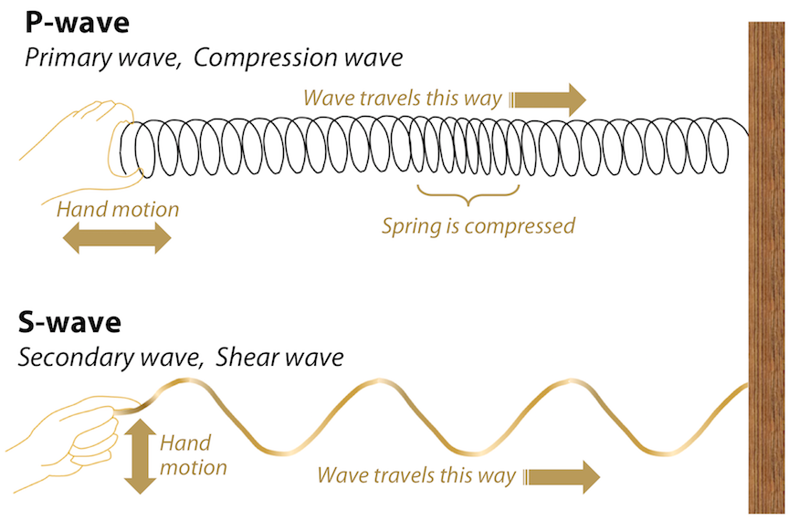
S-waves are body waves that move with a shearing motion, shaking particles from side to side. S-waves can be simulated by fixing one end of a rope to a solid surface, then giving the other end a flick (Figure 12.8, bottom). Any one point on the rope will move from side to side at a right angle to the direction in which the snaking motion is traveling. The “S” in S-wave stands for secondary, because S-waves are slower than P-waves, and are detected after the P-waves are measured. S-waves cannot travel through liquids.

P-waves and S-waves can travel rapidly through geological materials, at speeds many times the speed of sound in air.

Surface Waves

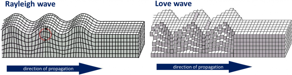
When body waves reach Earth’s surface, some of their energy is transformed into surface waves, which travel along Earth’s surface. Two types of surface waves are Rayleigh waves and Love waves (Figure 12.9). Rayleigh waves (R-waves) are characterized by vertical motion of the ground surface, like waves rolling on water. Love waves (L-waves) are characterized by side-to-side motion. Notice that the effects of both kinds of surface waves diminish with depth in Figure 12.9.

Surface waves are slower than body waves, and are detected after the body waves. Surface waves typically cause more ground motion than body waves, and therefore do more damage than body waves.

Concept Check: Seismic Wave Types

Fill in the blanks to complete this summary of types of seismic waves.

              -waves ( hint: P, S, R, or L?) are               ( hint: fast or slow?) body waves that move by compressing and stretching rock.

              -waves ( hint: P, S, R, or L?) are               ( hint: fast or slow?) body waves that move by shearing rock.

              -waves ( hint: P, S, R, or L?) are surface waves that produce a rolling motion.

              -waves ( hint: P, S, R, or L?) are surface waves that produce a side-to-side motion.

To check your answers, navigate to the below link to view the interactive version of this activity.

Recording Seismic Waves Using a Seismograph

A seismometer is an instrument that detects seismic waves. An instrument that combines a seismometer with a device for recording the waves is called a seismograph . The graphical output from a seismograph is called a seismogram . Figure 12.10 (right) shows how a seismograph works. The instrument consists of a frame or housing that is firmly anchored to the ground. A mass is suspended from the housing, and can move freely on a spring. When the ground shakes, the housing shakes with it, but the mass remains fixed. A pen attached to the mass moves up and down on a rotating drum of paper, drawing a wavy line, the seismogram. The seismograph in Figure 12.10 (right) is oriented to measure vertical ground motion. The photo on the left shows a seismograph oriented to record horizontal ground motion.

The pen and drum of a mechanical seismograph record the motion of the ground relative to the mass. However, unless an earthquake causes a large amount of ground motion directly beneath the seismograph, the height of the wave recorded on paper might be very small, making the seismogram difficult to analyze. The seismograph on the right has a device to amplify the ground motion, drawing larger waves that are easier to study.

Modern seismographs record shaking as electrical signals, and are able to transmit those signals. This means seismologists need not return to the instrument to collect recordings before the records can be examined.

Finding The Location of an Earthquake

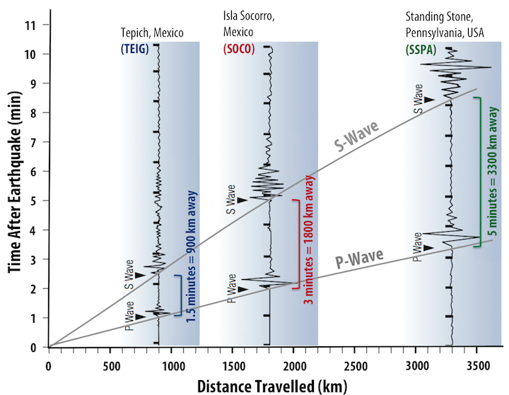
P-waves travel faster than S-waves. As the waves travel away from the location of an earthquake, the P-wave gets farther and farther ahead of the S-wave. Therefore, the farther a seismograph is from the location of an earthquake, the longer the delay between when the P-wave arrival is recorded, and the S-wave arrival is recorded. The delay between the P-wave and S-wave arrival appears as a widening gap in a diagram of P-wave and S-wave travel times (Figure 12.11, grey lines).

P-wave and S-wave arrival times can be identified on seismograms. In the three seismograms in Figure 12.11, the arrivals of the P-waves and S-waves are marked with arrows, and the interval in minutes between the P-wave and S-wave arrivals are noted. The seismograms were recorded at three different seismic stations (earthquake monitoring locations equipped with seismographs). The distance of each station from the earthquake is determined by finding the distance along the graph where the gap between the P-wave and S-wave travel-time curves matches the delay between P-wave and S-wave arrivals on the seismogram.

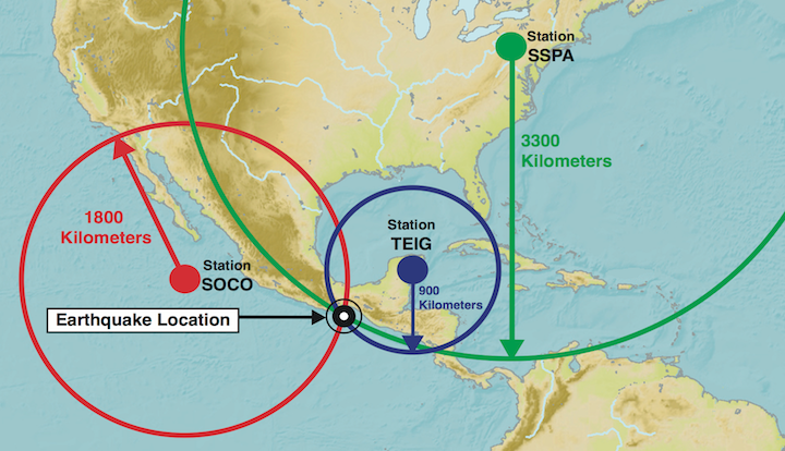
The delay between the P-wave and S-wave arrival at a seismic station can indicate how far the station is from the source of the earthquake, but not the direction the seismic waves came from. The possible locations of the earthquake can be represented on a map by drawing a circle around the seismic station, with the radius of the circle being the distance determined from the P-wave and S-wave travel times (Figure 12.12). If this is done for at least three seismic stations, the circles will intersect at the origin of the earthquake. This method is called triangulation .

Concept Check: Finding the Location of an Earthquake

Fill in the blanks to complete this description of how earthquakes are located by triangulation.

The               -waves ( hint: P or S) generated by an earthquake are faster than               -waves ( hint: P or S). The farther seismic waves have to travel before reaching a seismic                ( hint: a monitoring location with a seisometer), the more the fast waves will gain on the slow ones, and the longer we have to wait after the fast waves arrive to see the slow ones. We can use that lag to figure out how far away the earthquake was.

This information gives us the               ( hint: direction or distance?) to the earthquake, but not the               ( hint: direction or distance?). To find the actual location, we need the lag information measured from at least               ( hint: how many?) locations. Then we can draw a circle from each location with a radius that matches the               ( hint: direction or distance?) we figured out. The location of the earthquake is where all of the circles                ( hint: geometry term for crossing).

How Big Was It?

Earthquakes can be described in terms of their magnitude , which reflects the amount of energy released by the shaking. They can also be described in terms of intensity , which characterizes the impact of the shaking on people and their surroundings.

Earthquake Magnitude

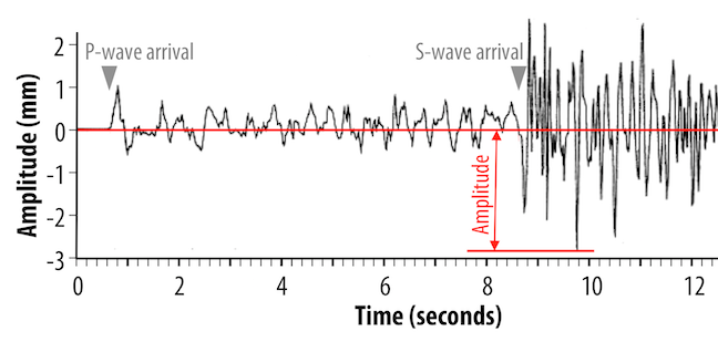
Earthquake magnitudes are determined by measuring the amplitudes of seismic waves. The amplitude is the height of the wave relative to the baseline (Figure 12.13). Wave amplitude depends on the amount of energy carried by the wave. The amplitudes of seismic waves reflect the amount of energy released by earthquakes.

The Richter magnitude scale uses the amplitudes of S-waves, and corrects for the decrease in amplitude that happens as the waves travel away from their source. The correction depends on how seismic waves interact with the specific rock types through which they travel, and therefore on local conditions, so the Richter magnitude is also referred to as the local magnitude .

While news reports about earthquakes might still refer to the “Richter scale” when describing magnitudes, the number they report is most likely the moment magnitude . The moment magnitude is calculated from the seismic moment of an earthquake. The seismic moment takes into account the surface area of the region that ruptured, how much displacement occurred, and the stiffness of the rocks. Moment magnitude can capture the difference between short earthquakes and longer ones resulting from larger ruptures, even of both types of earthquakes generate the same amplitude of waves. The moment magnitude scale is also better for earthquakes that are far from the seismic station. Seismic wave measurements are still used to determine the moment magnitude, however different waves are used than for the local magnitude scale.

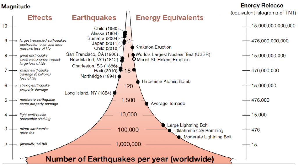
The magnitude scale is a logarithmic one rather than a linear one- an increase of one unit of magnitude corresponds to a 32 times increase in energy release (Figure 12.14). There are far more low-magnitude earthquakes than high-magnitude earthquakes. In 2017 there were 7 earthquakes of M7 (magnitude 7) or greater, but millions of tiny earthquakes.

Earthquake Intensity

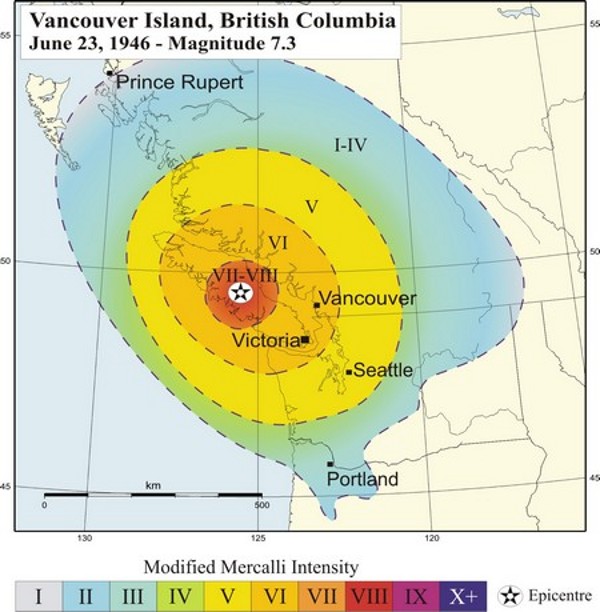
Intensity scales were first used in the late 19th century, and then adapted in the early 20th century by Giuseppe Mercalli and modified later by others to form what we now call the Modified Mercalli Intensity Scale (Table 12.1). To determine the intensity of an earthquake, reports are collected about what people felt and how much damage was done. The reports are then used to assign intensity ratings to regions where the earthquake was felt.

Intensity values are assigned to locations, rather than to the earthquake itself. This means that intensity can vary for a given earthquake, depending on the proximity to the epicentre and local conditions. For the 1946 M7.3 Vancouver Island earthquake, intensity was greatest in the central island region (Figure 12.15). In some communities within this region, chimneys were damaged on more than 75% of buildings. Some roads were made impassable, and a major rock slide occurred. The earthquake was felt as far north as Prince Rupert, as far south as Portland Oregon, and as far east as the Rockies, but with less intensity.

Intensity estimates are important as a way to identify regions that are especially prone to strong shaking. A key factor is the nature of the underlying geological materials. The weaker the underlying materials, the more likely it is that there will be strong shaking. Areas underlain by strong solid bedrock tend to experience far less shaking than those underlain by unconsolidated river or lake sediments.

An example of this effect is the 1985 M8 earthquake that struck the Michoacán region of western Mexico, southwest of Mexico City. There was relatively little damage near the epicentre, but 350 km away in heavily populated Mexico City there was tremendous damage and approximately 5,000 deaths. The reason is that Mexico City was built largely on the unconsolidated and water-saturated sediment of former Lake Texcoco. These sediments resonate at a frequency of about two seconds, which was similar to the frequency of the body waves that reached the city. Consequently, the shaking was amplified.  Survivors of the disaster recounted that the ground in some areas moved up and down by approximately 20 cm every two seconds for over two minutes. Damage was greatest to buildings between 5 and 15 storeys tall, because they also resonated at around two seconds, which amplified the shaking.

Try It: Modified Mercalli Intensity Scale

Ammon, C. J. (2001). Earthquake size . http://eqseis.geosc.psu.edu/~cammon/HTML/Classes/IntroQuakes/Notes/earthquake_size.html

• Source: U. S. Geological Survey (1989). The severity of an earthquake . USGS General Interest Publication, 1989-288-913 ↵

Physical Geology - H5P Edition Copyright © 2021 by Karla Panchuk is licensed under a Creative Commons Attribution-NonCommercial-ShareAlike 4.0 International License , except where otherwise noted.

Share This Book

• school Campus Bookshelves
• menu_book Bookshelves
• perm_media Learning Objects
• login Login
• how_to_reg Request Instructor Account
• hub Instructor Commons
• Download Page (PDF)
• Download Full Book (PDF)
• Periodic Table
• Physics Constants
• Scientific Calculator
• Reference & Cite
• Tools expand_more
• Readability

selected template will load here

This action is not available.

13.4: Locating an Earthquake Epicenter

• Last updated
• Save as PDF
• Page ID 5696

• Deline, Harris & Tefend
• University of West Georgia via GALILEO Open Learning Materials

During an earthquake, seismic waves are sent all over the globe. Though they may weaken with distance, seismographs are sensitive enough to still detect these waves. In order to determine the location of an earthquake epicenter, seismographs from at least three different places are needed for a particular event. In Figure 13.9, there is an example seismogram from a station that includes a minor earthquake. 

Once three seismographs have been located, find the time interval between the arrival of the P-wave and the arrival of the S-wave. First, determine the P-wave arrival, and read down to the bottom of the seismogram to note at what time (usually marked in seconds) that the P-wave arrived. Then do the same for the S-wave. The arrival of seismic waves will be recognized by an increase in amplitude – look for a pattern change as lines get taller and more closely spaced (ex. Figure 13.10).

By looking at the time between the arrivals of the P- and S-waves, one can determine the distance to the earthquake from that station, with longer time intervals indicating longer distance. These distances are determined using a travel-time curve, which is a graph of Pand S-wave arrival times (see Figure 13.11).

Though the distance to the epicenter can be determined using a travel-time graph, the direction cannot be told. A circle with a radius of the distance to the quake can be drawn. The earthquake occurred somewhere along that circle. Triangulation is required to determine exactly where it happened. Three seismographs are needed. A circle is drawn from each of the three different seismograph locations, where the radius of each circle is equal to the distance from that station to the epicenter. The spot where those three circles intersect is the epicenter (Figure 13.12).

9.2 Measuring Earthquakes

The shaking from an earthquake travels away from the rupture in the form of seismic waves . Seismic waves are measured to determine the location of the earthquake, and to estimate the amount of energy released by the earthquake (its magnitude ).

Types of Seismic Waves

Seismic waves are classified according to where they travel, and how they move particles.

Seismic waves that travel through Earth’s interior are called body waves . P-waves are body waves that move by alternately compressing and stretching materials in the direction the wave moves. For this reason, P-waves are also called compression waves. The “P” in P-wave stands for primary, because P-waves are the fastest of the seismic waves. They are the first to be detected when an earthquake happens.

A P-wave can be simulated by fixing one end of a spring to a solid surface, then giving the other end a sharp push toward the surface (Figure 9.8, top).  The compression will propagate (travel) along the length of the spring. Some parts of the spring will be stretched, and others compressed. Any one point on the spring will jiggle forward and backward as the compression travels along the spring.

S-waves are body waves that move with a shearing motion, shaking particles from side to side. S-waves can be simulated by fixing one end of a rope to a solid surface, then giving the other end a flick (Figure 9.8, bottom). Any one point on the rope will move from side to side at a right angle to the direction in which the snaking motion is traveling. The “S” in S-wave stands for secondary, because S-waves are slower than P-waves, and are detected after the P-waves are measured. S-waves cannot travel through liquids.

P-waves and S-waves can travel rapidly through geological materials, at speeds many times the speed of sound in air.

Surface Waves

When body waves reach Earth’s surface, some of their energy is transformed into surface waves, which travel along Earth’s surface. Two types of surface waves are Rayleigh waves and Love waves (Figure 9.9). Rayleigh waves (R-waves) are characterized by vertical motion of the ground surface, like waves rolling on water. Love waves (L-waves) are characterized by side-to-side motion. Notice that the effects of both kinds of surface waves diminish with depth in Figure 9.9.

Surface waves are slower than body waves, and are detected after the body waves. Surface waves typically cause more ground motion than body waves, and therefore do more damage than body waves.

Recording Seismic Waves Using a Seismograph

A seismometer is an instrument that detects seismic waves. An instrument that combines a seismometer with a device for recording the waves is called a s eismograph . The graphical output from a seismograph is called a seismogram . Figure 9.10 (right) shows how a seismograph works. The instrument consists of a frame or housing that is firmly anchored to the ground. A mass is suspended from the housing, and can move freely on a spring. When the ground shakes, the housing shakes with it, but the mass remains fixed. A pen attached to the mass moves up and down on a rotating drum of paper, drawing a wavy line, the seismogram. The seismograph in Figure 9.10 (right) is oriented to measure vertical ground motion. The photo on the left shows a seismograph oriented to record horizontal ground motion.

The pen and drum of a mechanical seismograph record the motion of the ground relative to the mass. However, unless an earthquake causes a large amount of ground motion directly beneath the seismograph, the height of the wave recorded on paper might be very small, making the seismogram difficult to analyze. The seismograph on the right has a device to amplify the ground motion, drawing larger waves that are easier to study.

Modern seismographs record shaking as electrical signals, and are able to transmit those signals. This means seismologists need not return to the instrument to collect recordings before the records can be examined.

Finding The Location of an Earthquake

P-waves travel faster than S-waves. As the waves travel away from the location of an earthquake, the P-wave gets farther and father ahead of the S-wave. Therefore, the farther a seismograph is from the location of an earthquake, the longer the delay between when the P-wave arrival is recorded, and the S-wave arrival is recorded. The delay between the P-wave and S-wave arrival appears as a widening gap in a diagram of P-wave and S-wave travel times (Figure 9.11, grey lines).

P-wave and S-wave arrival times can be identified on seismograms. In the three seismograms in Figure 9.11, the arrivals of the P-waves and S-waves are marked with arrows, and the interval in minutes between the P-wave and S-wave arrivals are noted. The seismograms were recorded at three different seismic stations (earthquake monitoring locations equipped with seismographs). The distance of each station from the earthquake is determined by finding the distance along the graph where the gap between the P-wave and S-wave travel-time curves matches the delay between P-wave and S-wave arrivals on the seismogram.

The delay between the P-wave and S-wave arrival at a seismic station can indicate how far the station is from the source of the earthquake, but not the direction from which the seismic waves travelled. The possible locations of the earthquake can be represented on a map by drawing a circle around the seismic station, with the radius of the circle being the distance determined from the P-wave and S-wave travel times (Figure 9.12). If this is done for at least three seismic stations, the circles will intersect at the origin of the earthquake.

How Big Was It?

Earthquakes can be described in terms of their magnitude , which reflects the amount of energy released by the shaking. They can also be described in terms of intensity , which characterizes the impact of the shaking on people and their surroundings.

Earthquake Magnitude

Earthquake magnitudes are determined by measuring the amplitudes of seismic waves. The amplitude is the height of the wave relative to the baseline (Figure 9.13). Wave amplitude depends on the amount of energy carried by the wave. The amplitudes of seismic waves reflect the amount of energy released by earthquakes.

The Richter magnitude scale uses the amplitudes of S-waves, and corrects for the decrease in amplitude that happens as the waves travel away from their source. The correction depends on how seismic waves interact with the specific rock types through which they travel, and therefore on local conditions, so the Richter magnitude is also referred to as the local magnitude .

While news reports about earthquakes might still refer to the “Richter scale” when describing magnitudes, the number they report is most likely the moment magnitude . The moment magnitude is calculated from the seismic moment of an earthquake. The seismic moment takes into account the surface area of the region that ruptured, how much displacement occurred, and the stiffness of the rocks. Moment magnitude can capture the difference between short earthquakes and longer ones resulting from larger ruptures, even of both types of earthquakes generate the same amplitude of waves. The moment magnitude scale is also better for earthquakes that are far from the seismic station. Seismic wave measurements are still used to determine the moment magnitude, however different waves are used than for the local magnitude scale.

The magnitude scale is a logarithmic one rather than a linear one- an increase of one unit of magnitude corresponds to a 32 times increase in energy release (Figure 9.14). There are far more low-magnitude earthquakes than high-magnitude earthquakes. In 2017 there were 7 earthquakes of M7 (magnitude 7) or greater, but millions of tiny earthquakes.

Earthquake Intensity

Intensity scales were first used in the late 19th century, and then adapted in the early 20th century by Giuseppe Mercalli and modified later by others to form what we now call the Modified Mercalli Intensity Scale (Table 9.1). To determine the intensity of an earthquake, reports are collected about what people felt and how much damage was done. The reports are then used to assign intensity ratings to regions where the earthquake was felt.

Intensity values are assigned to locations, rather than to the earthquake itself. This means that intensity can vary for a given earthquake, depending on the proximity to the epicenter and local conditions. For the 1946 M7.3 Vancouver Island earthquake, intensity was greatest in the central island region (Figure 9.15). In some communities within this region, chimneys were damaged on more than 75% of buildings. Some roads were made impassable, and a major rock slide occurred. The earthquake was felt as far north as Prince Rupert, as far south as Portland Oregon, and as far east as the Rockies, but with less intensity.

Intensity estimates are important as a way to identify regions that are especially prone to strong shaking. A key factor is the nature of the underlying geological materials. The weaker the underlying materials, the more likely it is that there will be strong shaking. Areas underlain by strong solid bedrock tend to experience far less shaking than those underlain by unconsolidated river or lake sediments.

An example of this effect is the 1985 M8 earthquake that struck the Michoacán region of western Mexico, southwest of Mexico City. There was relatively little damage near the epicenter, but 350 km away in heavily populated Mexico City there was tremendous damage and approximately 5,000 deaths. The reason is that Mexico City was built largely on the unconsolidated and water-saturated sediment of former Lake Texcoco. These sediments resonate at a frequency of about two seconds, which was similar to the frequency of the body waves that reached the city. Consequently, the shaking was amplified.  Survivors of the disaster recounted that the ground in some areas moved up and down by approximately 20 cm every two seconds for over two minutes. Damage was greatest to buildings between 5 and 15 stories tall, because they also resonated at around two seconds, which amplified the shaking.

Video: Geoscience Videos – Measuring Earthquakes

Ammon, C. J. (2001). Earthquake Size Visit website

Licenses and Attributions

“Physical Geology, First University of Saskatchewan Edition” by Karla Panchuk is licensed under CC BY-NC-SA 4.0 Adaptation: Renumbering

https://openpress.usask.ca/physicalgeology/

Principles of Earth Science Copyright © 2021 by Katharine Solada and K. Sean Daniels is licensed under a Creative Commons Attribution-NonCommercial-ShareAlike 4.0 International License , except where otherwise noted.

Share This Book

• Docs »
• Seismic »
• Basic principles »
• Travel times
• Edit on GitHub

Travel times ¶

A seismic wave travelling through an isotropic homogeneous medium will propagate at a constant velocity. Therefore, the time \(t\) required for a seismic wave to travel from source to receiver in a homogeneous earth layer with velocity \(v\) is simply given by the formula

where \(d\) is the distance travelled in the layer. In a seismic survey we measure source to receiver travel times and use those data to estimate the properties of the subsurface. Basic seismic interpretation methods assume that the earth is composed of a series of uniform layers and attempt to compute the thicknesses, velocities, and sometimes dips of each layer. We will discuss specific techniques for computing layer thicknesses and velocities in the reflection and refraction survey sections. However, we will introduce the concept of travel time computations and how they relate to geometry here, using the example of a two layered earth.

Consider a layer of thickness h and velocity \(v_1\) overlying a uniform halfspace of velocity \(v_2\) . A source is detonated at time \(t=0\) . We are interested in the waves and arrival times of those waves at a receiver which is located at a distance \(x\) from the source at position \(D\) in the figure below. There are three principal waves that will travel through the earth and arrive at position D. i) direct waves, ii) reflected waves, and iii) critically refracted waves.

The travel time curves for these ray paths are shown below, where the horizontal axis represents distance from the source along the flat surface of the earth, \(x_{crit}\) is called the critical distance, and \(x_{cross}\) the crossover distance. The critical distance is the closest surface point to the source at which the refracted ray can be observed. The crossover distance is the surface point at which the direct and refracted rays arrive at the same time. At offsets from the source greater than the crossover distance the refracted ray will be the first signal to arrive from the source. You can explore these concepts interactively using the Science seismic refraction app . Instructions for using the app can be found here . The following video illustrates the propagation of headwaves and how they relate to the crossover distance

Travel times of visible arrivals are related to the distance between source and receiver ( \(x\) ), thickness of the layer ( \(h\) ) and the wave velocities in the upper layer and basement ( \(v_1\) and \(v_2\) ). Let us denote the arrival times at point \(x\) for the direct, reflected and refracted waves as \(t_{dir}\) , \(t_{refl}\) \(t_{refr}\) respectively. These times are given by the following formulas

Note that the formulas for the direct and refracted waves are linear in \(x\) but that the reflected arrival time formula is not.

Before moving on, let’s look at an example of how travel times show up in the field. The horizontal axis of the following plot shows offset from a seismic receiver. Each line plots the displacement vs time curve of a geophone at a given offset. The plot clearly shows a set of events moving linearly in time from one geophone to the next.

We will now discuss the computation of traveltimes in more detail. It is important to note here that computing traveltimes for an arbitrary, heterogeneous earth is a complex problem well beyond the scope of this course. However, much insight can be gained by assuming that the subsurface consists of a series of homogeneous layers with horizontal or possibly dipping interfaces.

Refracted ray in a two layered-earth ¶

We need to identify specific ray paths and their associated travel times. Consider an earth composed of a uniform layer with velocity \(v_1\) and thickness \(z\) overlying a medium with velocity \(v_2\) . Let \(\theta\) be the critical angle and x denoted the distance between the source at \(A\) and a receiver at \(D\) . Let \(x_c\) denote the critical distance.

From elementary geometry the following relationships hold:

The travel time is the cumulative time for the wave to traverse the path \(ABCD\) . This is \(t=t_{AB}+t_{BC}+t_{CD}\) .

Generally time = distance / velocity, so we can write \(t_{AB} = L/v_1 = (z/cos\theta) / v1\) , (using \(L\) from just above).

Also, we can note that \(t_{AB} = t_{CD}\) and the distance \(BC\) is \(x-x_c\) . So we can now state that \(t=2t_{AB}+t_{BC}\) , or

It is convenient to rearrange this slightly differently. Using the definition for critical angle \(\sin\theta=v_1/v_2\) , we can make the “velocity triangle”, so expressions for the angle arise directly from simple trigonometry:

Use these two relations for \(\cos\) and \(\tan\) in the expression for t above to obtain a useful set of relations.

This simple relation says that the travel time curve is a straight line which has a slope of \(1/v_2\) and an intercept of \(t_i\) . This intercept time is the time where the refraction line extends to intercept the \(y\) -axis –above the source position–. This is not a real “time” - it is derived from the graph.

The velocities of the seismic layers and the layer thickness are obtained in the following manner.

Plot the times of first arrivals on an time-offset plot (“offset” is distance between source and geophone).

The direct arrivals are observed to lie along a straight line joining the origin. The slope of this line is \(1/v_1\) , giving the velocity of the upper layer.

The refracted arrivals appear as a straight line with smaller slope equal to \(1/v_2\) , giving the velocity of the lower layer.

For the refracted wave, this intercept time is

We therefore can obtain all three useful parameters about the earth, \((v_1, z, v_2)\) .

There is another useful point that is observable from the first arrival travel-time plot. We can often discern the crossover distance. Since this is the location where the direct wave and the refracted wave arrive at the same time, we can write

This can be used as a consistency check, or it can be used to compute one of the variables given values for two others.

Refracted ray in a three layered-earth ¶

The extension to more layers is in principle straight forward. Snell’s law holds for waves at all interfaces, so for a multi-layered medium

For a three layer case, the algebra is slightly more involved compared to a two layer example because we need to compute the times due to the ray path segments in the two top layers. Consider the diagrams below:

Using arguments that are entirely analagous to the two layer case (above) the travel time for the wave refracted at the top of layer three is given by

All quantities are defined in the diagrams, and the angles are

Note that \(\theta_2\) is a critical angle while \(\theta_1\) is not. You can prove the relation for \(\theta_1\) yourself by using Snell’s law at the two interfaces, and recalling that the angle of the ray coming from point \(B\) is the same as the angle arriving at point \(C\) . The straight line that corresponds to an individual refractor provides a velocity (from its slope) and a thickness (from the intercept). Thus the information on the above travel-time plot allows us to recover all three velocities and the thickness of both layers.

The travel time curves for multi layers are obtained from obvious extension of the above formulation.

Reflected rays - single layer ¶

Consider the situation to the right, in which there is a source \(S\) and a set of receivers on the surface of the earth. The earth is a single uniform layer overlying a uniform halfspace. A reflection from the interface will occur if there is a change in the acoustic impedance at the boundary.

Let \(x\) denote the “offset” or distance from the source to the receiver. The time taken for the seismic energy to travel from the source to the receiver is given by

\[t = \frac{(x^2 + 4z^2)^\frac{1}{2}}{v}\]

This is the equation of a hyperbola. In seismic reflection (as in radar) we plot time on the negative vertical axis, and so the seismic section (without the source wavelet) would look like.

Two way travel time:

Normal Moveout:

In the above diagram \(t_0\) is the 2-way vertical travel time. It is the minimum time at which a reflection will be recorded. The additional time taken for a signal to reach a receiver at offset \(x\) is called the “Normal Moveout” time, \(\Delta t\) . This value is required for every trace in the common depth point data set in order to shift echoes up so they align for stacking. How is it obtained? First let us find a way of determining velocity and \(t_0\) .

For this simple earth structure the velocity and layer thickness can readily be obtained from the hyperbola. Squaring both sides yields,

This is the equation of a straight line when \(t^2\) is plotted against \(x^2\) . Now, to find \(\Delta T\) , we must rearrange this hyperbolic equation relating \(t_0\) , \(x\) , the \(Tx\) – \(Rx\) offset, \(t\) at \(x\) , or \(t(x)\) , and the ground’s velocity, \(v\) .

Apply binomial expansion to get

Now, since normal moveout is \(\Delta T = t_x - t_0\)

The algebra has only one complicated step–a binomial expansion must be applied to obtain a simple relation without square roots etc.

The approximation is valid so long as the source-receiver separation (or offset) is “small” which means much less than the vertical depth to the reflecting layer (i.e. \(x << vt_0\) ). The result is a simple expression for normal moveout.

Each echo can be shifted up to align with the \(t_0\) position, so long as the trace position, \(x\) , the vertical incident travel time, \(t_0\) , and the velocity are known. Velocity can be estimated using the slope of the \(t^2\) – \(x^2\) plot, or with several other methods, which we will discuss in pages following.

Travel Time Curves for Multiple Layers ¶

If there are additional layers then the seismic energy at each interface is refracted according to Snell’s Law. The energy no longer travels in a straight line and hence the travel times are affected. It is observed that for small offsets, the travel time curve is still approximately hyperbolic, but the velocity, which controls the shape of the curve, is an “average” velocity determined from the velocities of all the layers above the reflector. The velocity is called the RMS (Root Mean Square) velocity, \(v_{rms}\) .

The complex travel path of a reflected ray through a multilayered ground. (b) The time–distance curve for reflected rays following the above type of path. Note that the divergence from the hyperbolic travel-time curve for a homogeneous overburden of velocity Vrms increases with offset.

As outlined in the figure above, the reflection curve for small offsets is still like a hyperbola, but the associated velocity is \(v_{rms}\) , not a true interval velocity.

For each hyperbola:

By fitting hyperbolas to each reflection event one can obtain \(t_n,v_n^{rms}\) for n = 1, 2, … The interval velocity and layer thickness of each layer can be found using the formulae below:

These formulae for the interval velocity and thickness of the \(n^{th}\) layer are directly obtainable from the definition of \(v_n^{rms}\) given above. The RMS velocity for the \(n^{th}\) layer is given by:

where \(v_i\) is the velocity of the \(i^{th}\) layer, and \(\tau_i\) is the one-way travel time through the \(i^{th}\) layer.

Powerful math software that is easy to use

• Maple Add-Ons

Advanced System Level Modeling

• MapleSim Add-Ons

Systems Engineering

• Consulting Services

Maple T.A. and Möbius

Automotive and Aerospace

Machine design & industrial automation.

• Application Areas
• Product Pricing
• Institutional Student Licensing
• Maplesoft Elite Maintenance (EMP)
• Product Training
• Online Product Help
• Webinars & Events
• Publications
• Content Hubs
• Examples & Applications
• About Maplesoft
• Media Center
• User Community

• Maple Learn
• Maple Calculator App
• System Engeneering
• Online Education Products

Online Help

All products    maple    maplesim.

The second type of wave to consider when determining the epicenter of an earthquake is the S-wave . These waves are also referred to as secondary or shear waves. S-waves can also be characterized by some unique properties:

The following animation helps to understand the motion of each type of wave.

A seismogram  is the graph output from a seismograph , which is used to determine the epicenter of an earthquake. When consulting the seismogram, P-waves always appear before S-waves, as they travel faster and can travel through three states of matter as opposed to one.

To determine the distance of an earthquake epicenter:

Suppose the P-wave arrives at t  = 1.0 min and the S-wave arrives at t  = 6.0 min. Determine the distance of the earthquake epicenter given the following information.

Download Help Document

Download a Free Trial of Maple

Try Maple free for 15 days with no obligation.

Maple 2024 now available.

Save an additional 20% on Maple 2024 Upgrades until March 31, 2024.

Copyright © 2001 Virtual Courseware for Earth and Environmental Sciences

How Often Do Earthquakes Happen in the Northeast?

A 4.8 magnitude earthquake that struck New Jersey Friday morning was felt from Baltimore to New York City , leaving residents rattled by the seismic activity that rarely happens in the area. But experts say people should not be concerned that quakes will happen more frequently along the eastern U.S.

“There's no clear trend that there are more earthquakes happening,” Angie Lux, a seismologist working at the University of California Berkeley Seismology Lab, tells TIME. 

Since 1950, about 40 earthquakes measuring magnitudes 3 or larger have hit within 500 km, or about 310 miles, of Friday’s earthquake, which struck near Whitehouse Station, N.J. at 10:23 a.m. ET, according to the United States Geological Survey (USGS). The last earthquake of similar magnitude to impact the region was in 2011, when a 5.8 quake struck central Virginia but was also felt across the East Coast. That quake caused property damage between $200 to $300 million and was likely felt by more people than any other earthquake in North American history.

Lingsen Meng, a geophysics associate professor at the University of California Los Angeles, says that earthquakes are uncommon along the East Coast, and advises people to stay calm. “Small earthquakes occur much more often than big ones,” he says. The largest earthquakes that have struck along the East Coast were the 1755 Cape Ann earthquake in Boston, and a 7.2 quake in Charleston, S.C. in 1886.

Read More : New York City Rattled by 4.8 Magnitude Earthquake

“It [was] much bigger than the ones we have today,” Meng adds.

USGS research social scientist Sarah McBride told reporters during a Friday afternoon call that the organization has recorded at least two aftershocks related to Friday’s earthquake, but added that there’s only a 3% chance of an aftershock with a magnitude five or greater in the coming weeks.

What caused the earthquake?

Earthquakes typically happen when there’s movement between tectonic plates, which are the plates that make up the earth’s crust. That’s why states like California, which straddles the San Andreas fault, experience earthquakes more frequently.

Friday’s earthquake did not happen at an active fault, USGS says. “There are dozens of older inactive faults that formed millions of years ago. And under the current stresses from tectonic plates moving those faults can be intermittently reactivated,” a USGS spokesperson told press on Friday. She added that scientists still had to do more research to understand why the event occurred.

Meng says that people should not stress too much about potential infrastructure damage. “Building damage usually doesn't happen until [magnitude] six or seven. So [today’s earthquake] is not going to cause any significant damage unless the building is really inadequate.”

Read More : Meet the Eclipse Chasers Traveling Thousands of Miles for the Astronomical Event

The only factor that might be cause for concern has to do with the seismic waves traveling across the East Coast, which are felt more widely because of differences in the Earth’s crust. “East Coast seismic waves tend to travel much longer distances. They don't attenuate or decay as fast,” Meng says. “So you might feel the earthquakes over a longer distance but consider these big earthquakes are very rare in the East Coast so the likelihood of having big damage or building collapse is still low.”

More Must-Reads From TIME

• The 100 Most Influential People of 2024
• The Revolution of Yulia Navalnaya
• 6 Compliments That Land Every Time
• What's the Deal With the Bitcoin Halving?
• If You're Dating Right Now , You're Brave: Column
• The AI That Could Heal a Divided Internet
• Fallout Is a Brilliant Model for the Future of Video Game Adaptations
• Want Weekly Recs on What to Watch, Read, and More? Sign Up for Worth Your Time

Contact us at [email protected]

• Software-web-app
• Seismic waves viewer
• Fact-Sheets
• Software-Web-Apps

Seismic Waves Viewer Open

Seismic Waves is a browser-based tool to visualize the propagation of seismic waves from historic earthquakes through Earth’s interior and around its surface. Easy-to-use controls speed-up, slow-down, or reverse the wave propagation. By carefully examining these seismic wave fronts and their propagation, the Seismic Waves tool illustrates how earthquakes can provide evidence that allows us to infer Earth’s interior structure.

Shear waves (S waves), for example, travel through the Earth at approximately one-half the speed of compression waves (P waves). Stations close to the earthquake record strong P, S, and Surface waves in quick succession just after the earthquake occurred. Stations farther away record the arrival of these waves after a few minutes, and the times between the arrivals are greater. 

The tool also illustrates how seismic waves inform our current understanding of Earth’s interior structure. Users will see that between approximately 104 and 140 degrees away from the epicenter, direct P waves do not arrive as they are refracted away from this zone. This suggests the presence of a lower velocity material, Earth’s outer core. Users will also observe that no direct S waves arrive beyond 104 degrees. 

This web-based Seismic Waves Viewer mirros the functionality of the original Seismic Waves tool  produced through a collaboration between Alan Jones & Jeff Baker ( Binghamton University ) and IRIS EPO. The original Seismic Waves runs on MS-Windows on PCs ( Download .exe file here ). You can learn more about Seismic Waves here. Jones, A. (2005). Using the Seismic Waves Program to Illustrate Wave Propogation Through the Earth. The Earth Scientist, 21(2), 26-27. 

• Seismic Waves Viewer —TUTORIAL Video Novice Seismic Waves is a browser-based tool to visualize the propagation of seismic waves from historic earthquakes through Earth’s interior and around its surface.

Related Fact-Sheets

Earthquakes create seismic waves that travel through the Earth. By analyzing these seismic waves, seismologists can explore the Earth's deep interior. This fact sheet uses data from the 1994 magnitude 6.9 earthquake near Northridge, California to illustrate both this process and Earth's interior structure.

NOTE: Out of Stock; self-printing only.

Related Videos

Video lecture on wave propagation and speeds of three fundamental kinds of seismic waves.

Related Animations

Seismic waves travel through the earth to a single seismic station. Scale and movement of the seismic station are greatly exaggerated to depict the relative motion recorded by the seismogram as P, S, and surface waves arrive.

We use exaggerated motion of a building (seismic station) to show how the ground moves during an earthquake, and why it is important to measure seismic waves using 3 components: vertical, N-S, and E-W. Before showing an actual distant earthquake, we break down the three axes of movement to clarify the 3 seismograms. 

Seismic shadow zones have taught us much about the inside of the earth. This shows how P waves travel through solids and liquids, but S waves are stopped by the liquid outer core.

The wave properties of light are used as an analogy to help us understand seismic-wave behavior.

The shadow zone is the area of the earth from angular distances of 104 to 140 degrees from a given earthquake that does not receive any direct P waves. The different phases show how the initial P wave changes when encountering boundaries in the Earth.

The shadow zone results from S waves being stopped entirely by the liquid core. Three different S-wave phases show how the initial S wave is stopped (damped), or how it changes when encountering boundaries in the Earth. 

Seismic tomography is an imaging technique that uses seismic waves generated by earthquakes and explosions to create computer-generated, three-dimensional images of Earth's interior. CAT scans are often used as an analogy. Here we simplify things and make an Earth of uniform density with a slow zone that we image as a magma chamber.

A travel time curve is a graph of the time that it takes for seismic waves to travel from the epicenter of an earthquake to the hundreds of seismograph stations around the world. The arrival times of P, S, and surface waves are shown to be predictable. This animates an IRIS poster linked with the animation.

Related Software-Web-Apps

Related Posters

Seismic waves from earthquakes ricochet throughout Earth's interior and are recorded at geophysical observatories around the world. The paths of some of those seismic waves and the ground motion that they caused are used by seismologists to illuminate Earth's deep interior.

We encourage the reuse and dissemination of the material on this site as long as attribution is retained. To this end the material on this site, unless otherwise noted, is offered under Creative Commons Attribution ( CC BY 4.0 ) license

• Mailing Lists
• Frequently Asked Questions
• Privacy Policy
• Terms of Service
• Comments about this page
• Instrumentation Services
• Data Services

Tsunami alert after volcano in Indonesia erupts, thousands told to leave

Indonesian authorities issued a tsunami alert on Wednesday after eruptions at Ruang mountain sent ash thousands of feet high.

Officials ordered more than 11,000 people to leave the area.

The volcano on the northern side of Sulawesi island had at least five large eruptions in the past 24 hours, Indonesia's Center for Volcanology and Geological Disaster Mitigation said.

Authorities raised their volcano alert to its highest level.

There were no reports of deaths or injuries.

The National Disaster Management Agency's spokesperson Abdul Muhari told ABC that residents have been moving to the east part of Tagulandang Island.

"They have been moving to the north and east area," he said.

"But we aren't able to reveal the numbers yet … because the rock ejection is still happening and we are prioritising staff's safety."

Mr Muhari said until Thursday morning local time, the volcanic ash has "subsided but the volcanic ash is quite spread out".

"We couldn't land in the local airport," he said.

"Our team would have to wait until the airport is open."

At least 800 residents were evacuated from two Ruang Island villages to nearby Tagulandang Island, according to an earlier report by state agency.

Indonesia, an archipelago of 270 million people, has 120 active volcanoes.

It is prone to volcanic activity because it sits along the 'Ring of Fire', a horseshoe-shaped series of seismic fault lines around the Pacific Ocean.

The volcanology agency said on Tuesday that volcanic activity had increased at Ruang after two earthquakes in recent weeks.

Authorities urged tourists and others to stay at least 6 kilometres from the 725-metre Ruang volcano.

Officials worry that part of the volcano could collapse into the sea and cause a tsunami similar to a 1871 eruption there.

In a press conference on Thursday, head of Indonesia's volcanology agency Hendra Gunawan said his team will evacuate more people to avoid casualties.

"Some people have been hit by the stones and got their heads scarred although not significant," he said.

"This however shows that the eruption is getting more intense."

Tagulandang island to the volcano's north-east is again at risk, and its residents are among those being told to evacuate.

Indonesia's National Disaster Mitigation Agency said residents will be relocated to Manado, the nearest city, on Sulawesi island, a journey of 6 hours by boat.

In 2018, the eruption of Indonesia's Anak Krakatau volcano caused a tsunami along the coasts of Sumatra and Java after parts of the mountain fell into the ocean, killing 430 people.

• X (formerly Twitter)

Related Stories

Foul-smelling sulphur and the risk of death won't stop tourists from climbing indonesia's active volcanoes.

Climbers killed, survivors found after Indonesian volcano erupts

Indonesia's Mount Merapi volcano spews rock, lava and gas 7km high

• Disasters, Accidents and Emergency Incidents
• Volcanic Eruptions

Advertisement

Supported by

Turkey Earthquake Trial Opens Amid Anger and Tears

More than 300 people were killed when temblors toppled an upscale residential complex. Survivors hope a court will punish the men who built it.

• Share full article

By Safak Timur and Ben Hubbard

Safak Timur reported from the courtroom in Antakya, Turkey, and Ben Hubbard from Istanbul.

The families addressed the court one by one, sobbing as they spoke the names of relatives who had been killed when their upscale apartment complex in southern Turkey toppled over during a powerful earthquake last year.

One woman, whose son had died in the collapse alongside his wife and their 3-year-old son, lashed out at the defendants — the men who had built the complex and the inspectors charged with ensuring that it was safe.

“Shame on you,” said the woman, Remziye Bozdemir. “Your children are alive, mine are dead.”

The hearing on Thursday was the first aimed at seeking accountability for the collapse of Renaissance Residence, one of the most catastrophic building failures during the earthquakes of Feb. 6, 2023 , which damaged hundreds of thousands of structures and killed more than 53,000 people across southern Turkey.

More than 300 people died inside Renaissance, and many more were wounded. An investigation and forensic analysis by The New York Times found that a tragic combination of poor design and minimal oversight had left the building vulnerable, ultimately causing its 13 stories to smash into the earth.

Since the quakes, the anger of many survivors has centered on the lax construction practices that allowed so many defective buildings to rise across a region with a history of powerful temblors. When the ground shook last year, many structures became death traps, pancaking down on their residents and killing them instantly or trapping them alive inside the rubble .

In recent months, Turkish courts have begun hearing cases seeking to assign responsibility for the deadly collapses. The Renaissance trial is one such case, which illustrates what victims’ advocates say are the limits of post-quake justice.

Eight men — four from the construction company and four employees of a private building-inspection firm — stand accused of causing foreseeable death and injury through negligence for their roles in the construction of the complex. All eight have pleaded not guilty.

Missing from the case are any of the numerous public officials who allowed the complex to be built by zoning the land, approving building plans and issuing construction permits, together failing to ensure that the project had been constructed to withstand violent quakes.

This scrutiny of private builders but not of public officials has marred efforts to ensure accountability across the quake zone, said Emma Sinclair-Webb, the Turkey director for Human Rights Watch.

“Contractors can be cowboy builders, building defective buildings, but what about the enabling environment in which they operate and the public authorities that turn a blind eye and let them go ahead?” she said.

Complicating efforts to hold such officials accountable is a Turkish law that prevents prosecutors from investigating state employees without obtaining government permission.

It remains unclear whether any public officials are on trial in earthquake-related cases.

In January, Human Rights Watch and Citizens’ Assembly , a Turkish rights group, filed requests in dozens of jurisdictions seeking information about how many requests to investigate public officials had been made and how many had been granted. Their queries turned up four instances in which decisions were pending and three in which permission to investigate had been granted, although two of those had been appealed, the groups said in a report last month.

Most jurisdictions declined to respond, citing confidentiality regulations.

This diminishes the chances for true accountability, Ms. Sinclair-Webb said.

“The full facts are not really there to be looked at if the public officials are left out of the picture,” she said.

Renaissance Residence rose on a patch of converted agricultural land near the ancient city of Antakya during a construction boom that was sweeping through the area in the 2010s, fueled by the plans of Turkey’s leader, Recep Tayyip Erdogan, for development and economic growth. By the time residents arrived in 2013, the three apartment towers, superficially joined to appear as one long, thin building, loomed over the countryside.

The complex catered to the area’s rising middle class, with a pool, underground parking and a lobby designed to mimic that of a hotel. Many early occupants considered themselves lucky to live there.

But The Times’s investigation found that, despite its air of glamour, Renaissance was rife with risky design choices that were cast in concrete with minimal oversight, leaving the structure ill prepared to withstand a powerful earthquake.

The first such quake stuck last year, with a magnitude of 7.8, followed by a second powerful temblor hours later. The first quake caused the ground floor of Renaissance to fail, making the building topple on its side and destroying many of its residents’ lives.

Cemile Incili, 59, a real estate agent who attended the hearing on Thursday, said she had survived the collapse with some injuries but had been able to hear her nephew trapped in the rubble.

“Aunt, I can’t breathe,” she recalled him saying.

His body, and that of a sister of Ms. Incili, were never recovered from the wreckage. She assumes they are dead.

She hoped the trial would mean long sentences for the men who built Renaissance as well as for the officials who allowed the building to rise.

“The state did not protect our lives or our property,” she said.

Court documents say that 269 people have been identified as having been killed in the building and that 46 others are still missing and assumed to be dead.

Prosecutors have charged the eight defendants with conscious negligence that caused multiple deaths and injuries. If convicted, they could face up to 22 years in prison.

The prosecutors have accused the contractors who built Renaissance of failing to follow the building codes in place at the time, using substandard materials and neglecting to ensure that the structure was sound. They have accused the inspectors, who worked for a private company hired by the contractors, of failing to detect flaws that should have been reported to the authorities.

The contractor who was the construction company’s lead architect, Mehmet Yasar Coskun, told the court on Thursday that he rejected the allegations. He blamed the collapse on the exceptional power of the earthquake’s shaking at the site.

“As the foundation of the building was strong, the wave demolished it from the weakest point it could find, the ground floor,” he said. “It is an atypical situation.”

Other defendants, too, said they had followed all the necessary regulations and attributed the collapse to the earthquake’s strength.

Their arguments failed to convince the survivors who attended the hearing.

Hafize Acikgoz, 42, had made it out of Renaissance alive but lost her husband and three children, who were 16, 21 and 23.

“It is just me left behind,” she said, wiping away tears. “Nothing can sooth my pain and nothing can bring them back.”

Still, she hoped that the accused would receive the longest possible sentences.

“Shouldn’t those buildings have been built considering people’s lives?” she said.

Beril Eski contributed reporting from Istanbul.

Ben Hubbard is the Istanbul bureau chief, covering Turkey and the surrounding region. More about Ben Hubbard